---
title: "Parametric bootstrap power analysis for multilevel ordinal EMA designs"
description: |
Design-oriented power analysis built on the modelling layer of phases
15a–15c. Generates ordinal multilevel EMA outcomes under hypothesised
within-subject effect magnitudes, with the random-intercept variance
and ordinal thresholds calibrated on the M0 fit from phase 15c
(latent-scale outcome ICC = 0.567 from M0 clmm; this is distinct from
the larger Bayesian ICC reported in phase 15c §3.5, see methodological
note in §2). Combines a hypothesis-driven design grid (n_subjects ×
n_emas × β_wz, 224 cells × 1000 replicates) refit with clmm, and a
brms-anchored sanity check that propagates posterior uncertainty from
the ADARP fit through the simulation. Reports power curves and
minimum detectable effects (MDE) per design cell, with practical
implications for ambulatory psychophysiology protocols in clinical
populations.
date: 2026-04-22
categories: [R, Power Analysis, Parametric Bootstrap, Multilevel Modelling, Ordinal Regression, Bayesian, brms, clmm, Simulation, EMA, ADARP]
execute:
echo: true
warning: false
message: false
freeze: auto
format:
html:
code-tools: true
code-fold: false
toc: true
toc-depth: 3
number-sections: true
theme: cosmo
fig-cap-location: bottom
embed-resources: false
---
```{r}
#| label: setup
#| code-summary: "Paths, packages, helpers, calibration anchors from phase 15c"
#| include: false
PROJECT_DIR <- normalizePath(
file.path("..", "files", "projet_25"),
mustWork = FALSE
)
DATA_MODE <- "processed" # or "demo"
DATA_DIR <- file.path(PROJECT_DIR, "data", DATA_MODE)
# Set to TRUE to force a full re-run of the simulation grid (~1-2 h on HPC).
# Default FALSE so the .qmd renders fast from cached parquet on subsequent
# runs.
FORCE_RERUN <- FALSE
suppressPackageStartupMessages({
library(arrow)
library(dplyr)
library(tidyr)
library(ggplot2)
library(knitr)
library(kableExtra)
library(patchwork)
library(MASS) # mvrnorm for correlated feature generation
library(ordinal) # clmm: frequentist cumulative-link mixed models
library(brms) # Bayesian multilevel models, posterior anchor
library(broom.mixed)
library(future)
library(furrr)
})
# select() is masked by MASS once it is loaded — we always use dplyr::select()
# explicitly downstream to avoid the silent column-vector return that MASS
# defaults to for character arguments.
select <- dplyr::select
source(file.path(PROJECT_DIR, "R", "render_helpers.R"))
theme_set(theme_minimal(base_size = 11))
# Top-10 features pre-specified for MLM in phase 15c. We only need the WZ
# block here: the BM block did not contribute to fit in phase 15c (M1 → M2
# LRT non-significant), so we simulate _wz effects only and set _bm to zero
# in the data-generating process.
TOP10_WZ <- c(
"hrv_rmssd_wz",
"hrv_hf_wz",
"eda_scl_mean_wz",
"eda_scr_rate_per_min_wz",
"acc_magnitude_std_wz"
)
```
```{r}
#| label: parallel-plan
#| code-summary: "Configure the future/furrr parallel backend"
#| include: false
# Parallelisation strategy: parallelise *within* each design cell (across
# the R replicates), not across cells. This keeps the resume-from-cache
# logic intact (one parquet flush per cell) and amortises worker spin-up
# over R = 1000 fits per cell, which is plenty.
#
# Set N_WORKERS based on the host. Leaves one core for the OS / Quarto
# render itself. On a 16-core HPC node, this gives 15 workers, which
# brings the Track 1 grid runtime down from ~1-2h serial to ~10-15 min.
# Set N_WORKERS = 1 to fall back to a serial sequential plan (useful
# for debugging the engine on a single replicate).
# On a desktop, leave 2 cores for the OS + browser/IDE rather than 1.
# Cap at 12 workers: beyond that, multisession overhead and RAM
# pressure (each worker copies the workspace) tend to dominate gains
# on a single machine.
N_WORKERS <- min(12L, max(1L, parallel::detectCores() - 2L))
if (N_WORKERS > 1L) {
plan(multisession, workers = N_WORKERS)
} else {
plan(sequential)
}
cat("Parallel plan: ", class(plan())[1],
" with ", nbrOfWorkers(), " worker(s)\n", sep = "")
```
`r data_mode_banner(DATA_DIR)`
---
## 1. From a null result to a design question
Phase 15c modelled the ADARP ordinal stress composite (`stress_composite`,
0–3) on n = 44 EMA windows clustered in 7 subjects, using a hierarchy
of cumulative-link mixed models. Three findings shaped this phase:
1. **No fixed-effect block significantly improved over the null
random-intercept model** at conventional α (LRTs M0 → M1 → M2 → M3
all non-significant; Hessian instability above M2 forced selection
of a model with stable variance-covariance for inference).
2. **The outcome ICC depends on which estimate one queries.** The
frequentist M0 clmm yields a latent-scale ICC of 0.567 (σ_u² = 4.31,
residual = π²/3); the best Bayesian model in 15c §3.5, evaluated by
`performance::icc()` after fixed effects, reports an adjusted ICC
of approximately 0.88. The two figures answer different questions
(raw variance partitioning of the outcome vs share of *residual*
variance attributed to subject after accounting for the best
fixed-effect structure under weakly informative priors) and are
not interchangeable. The simulator below uses the M0-clmm ICC of
0.567 as its calibration anchor, since it characterises the
data-generating structure prior to any injected effect — see the
methodological note in §2 for the full reasoning.
3. **LightGBM in the predictive track departed from the subject-mean
baseline** (weighted κ moved from −0.67 to +0.15), with DALEX
permutation importance ranking the EDA tonic block (`eda_scl_mean_wz`,
`eda_scl_slope_wz`) at the top — directionally consistent with the
autonomic-stress literature and with Alinia et al. (2021)'s day-level
correlations on the full ADARP collection.
Read together, these results are not "no signal". They are *signal at
a magnitude too small to clear conventional inferential thresholds at
n = 44 / 7*. The natural follow-on for a research-engineer deliverable
is to convert that observation into **design guidance**: at what cohort
size and EMA density would the same effect magnitude become detectable
at 80 % power?
This phase 15d builds that guidance through a parametric bootstrap.
Two parallel tracks meet at a single MDE table:
- **Track 1 — hypothesised effect grid.** For a fixed grid of
effect magnitudes `β_wz ∈ {0.1, …, 1.0}` log-odds applied uniformly
to the five WZ predictors, with random-intercept variance and
ordinal thresholds calibrated on the M0 fit from phase 15c, simulate
ordinal EMA datasets across `n_subjects × n_emas` design cells and
measure the proportion of replicates where a likelihood-ratio test
M0 vs M1 rejects at α = 0.05.
- **Track 2 — brms-anchored sanity check.** Refit M1 (WZ block only)
with brms on the ADARP n = 44 sample, sample 200 draws from the
joint posterior of (β_wz, σ_u), and propagate that uncertainty
through the simulation engine on a small set of diagnostic cells.
Yields a credibility band around the deterministic power curves of
Track 1.
Stack-wise, this notebook is **R-only**: every operation downstream
(`MASS::mvrnorm` for correlated-feature generation, `ordinal::clmm`
for the inferential test, `brms` for the Bayesian anchor) maps
naturally onto R packages with no signal-processing or ML pipeline
that would justify dropping into Python. This contrasts with phase 15a
(Empatica E4 ingestion, EDA non-wear detection — Python via parquet
hand-off) and 15b (cvxEDA convex-optimisation decomposition — same
pattern), where Python earned its place. Here, R is the domain-native
choice.
## 2. Generative model and calibration
We simulate ordinal outcomes from a cumulative-link mixed model with
a logit link:
$$
P(Y_{ij} \le k) = \text{logit}^{-1}(\theta_k - \eta_{ij}), \qquad
\eta_{ij} = \mathbf{x}_{ij}^\top \boldsymbol{\beta} + u_j,
$$
with $u_j \sim \mathcal{N}(0, \sigma_u^2)$ the subject-level random
intercept, $k \in \{0, 1, 2\}$ the three ordinal thresholds for a 4-level
outcome, and $\mathbf{x}_{ij}$ the 5-vector of within-subject
z-scored physiological features.
Three quantities are calibrated on the ADARP M0 fit from phase 15c
rather than fixed by hypothesis: the ordinal thresholds $\theta_k$,
the random-intercept variance $\sigma_u^2$, and the empirical
covariance structure of $\mathbf{x}_{ij}$.
```{r}
#| label: load-modelling-data
#| code-summary: "Re-load and re-build the phase 15c modelling dataset"
features_path <- file.path(DATA_DIR, "physio_features.parquet")
stopifnot(file.exists(features_path))

feat_all <- read_parquet(features_path)

mod_df <- feat_all %>%
  filter(usable_final == TRUE,
         feature_usable == TRUE,
         !is.na(stress_composite))

# Same n=2 minimum as phase 15c (Bolger & Laurenceau 2013): subjects with
# fewer than 2 EMAs are dropped because within-subject z-scoring requires
# at least two observations to estimate a within-person standard deviation.
subj_n <- mod_df %>% count(subject_id, name = "n_emas")
excluded_subjects <- subj_n %>%
  filter(n_emas < 2) %>%
  pull(subject_id)

mod_df <- mod_df %>%
  filter(!(subject_id %in% excluded_subjects)) %>%
  mutate(
    # Drop unobserved levels: phase 15c filtering retains categories
    # {1, 2, 3} only (category 0 has zero observations after the
    # usable_final ∧ feature_usable ∧ n≥2 chain). Passing an ordered
    # factor with levels = 0:3 to clmm causes silent threshold-dropping
    # in some versions and an outright error in others; we use only
    # the observed levels here.
    stress_composite_ord = factor(
      stress_composite,
      levels  = sort(unique(stress_composite)),
      ordered = TRUE
    ),
    subject_f = factor(subject_id)
  )

cat("  Categories observed       : ",
    paste(levels(mod_df$stress_composite_ord), collapse = ", "),
    "\n", sep = "")
cat("Modelling sample reconstructed from phase 15c:\n")
cat(" n_obs : ", nrow(mod_df), "\n", sep = "")
cat(" n_subjects : ", length(unique(mod_df$subject_id)), "\n", sep = "")
cat(" Excluded subjects (n<2) : ", paste(excluded_subjects, collapse = ", "), "\n", sep = "")
```
```{r}
#| label: refit-m0-anchor
#| code-summary: "Refit M0 (null random-intercept clmm) for parameter calibration"
m0_clmm <- clmm(
  stress_composite_ord ~ 1 + (1 | subject_f),
  data = mod_df,
  link = "logit"
)

# Ordinal thresholds θ_k (k = 0|1, 1|2, 2|3 on the latent log-odds scale)
thresholds_obs <- coef(m0_clmm)
cat("Ordinal thresholds (latent logit scale):\n")
print(round(thresholds_obs, 3))
# Random-intercept variance σ_u² (between-subject, latent logit scale)
sigma_u2_obs <- as.numeric(VarCorr(m0_clmm)$subject_f[1])
sigma_u_obs  <- sqrt(sigma_u2_obs)

# Outcome ICC (latent-scale): residual variance for a logistic link is
# fixed at π²/3, so ICC = σ_u² / (σ_u² + π²/3).
icc_outcome <- sigma_u2_obs / (sigma_u2_obs + pi^2 / 3)

cat("\nRandom-intercept SD σ_u    : ", round(sigma_u_obs, 3), "\n", sep = "")
cat("Random-intercept variance : ", round(sigma_u2_obs, 3), "\n", sep = "")
cat("Outcome ICC (latent scale) : ", round(icc_outcome, 3), "\n", sep = "")
```
```{r}
#| label: feature-covariance-anchor
#| code-summary: "Empirical covariance of the five WZ predictors"
X_obs <- as.matrix(mod_df[, TOP10_WZ])
Sigma_X_obs <- cov(X_obs, use = "complete.obs")
mu_X_obs    <- colMeans(X_obs, na.rm = TRUE)

# Diagonal of the covariance: should be close to 1 since these are
# within-subject z-scores; off-diagonal is the structure we want to
# preserve in the simulated features (e.g. RMSSD and HF are physiologically
# correlated; SCL_mean and SCR_rate share sympathetic activation).
cat("Empirical covariance Σ_X of the five WZ predictors:\n")
print(round(Sigma_X_obs, 2))
cat("\nDiagonal (within-subject z-score variances; expected ≈ 1):\n")
print(round(diag(Sigma_X_obs), 2))
```
The departures from unit variance on the diagonal are expected: the
within-subject z-score is computed using each subject's own mean and SD
on the *raw* feature distribution, but the pooled-sample variance of
the resulting `_wz` column reflects a mix of within-subject scaling
and the unequal cluster sizes that phase 15c kept (subject 111
contributes 16 EMAs, subject 106 contributes 2). The covariance
*structure* is what we propagate into the simulator; the diagonal
deviations are informative and kept as-is.
```{r}
#| label: calibration-summary
#| code-summary: "Calibration summary table"
#| echo: false
# The number of thresholds equals K = (n_categories - 1). After 25c
# filtering, the modelling sample contains only categories {1, 2, 3}
# of stress_composite (category 0 is absent — distribution 3/15/26
# across n = 44 obs), so clmm estimates two thresholds (1|2 and 2|3)
# rather than three. We label them accordingly.
K_obs <- length(thresholds_obs)
calib_tbl <- tibble::tibble(
Quantity = c(
sprintf("Ordinal threshold θ_1 (1|2)"),
sprintf("Ordinal threshold θ_2 (2|3)"),
"Random-intercept SD σ_u",
"Random-intercept variance σ_u²",
"Outcome ICC (latent logit scale, M0 clmm)"
),
Value = c(
round(thresholds_obs[1], 3),
round(thresholds_obs[2], 3),
round(sigma_u_obs, 3),
round(sigma_u2_obs, 3),
round(icc_outcome, 3)
),
Source = c(
"M0 clmm (phase 15c)",
"M0 clmm (phase 15c)",
"M0 clmm (phase 15c)",
"Derived from σ_u",
"σ_u² / (σ_u² + π²/3)"
)
)
calib_tbl %>%
kbl(caption = "Calibration anchors for the simulator, all derived from the phase 15c null model.") %>%
kable_styling(full_width = FALSE)
```
**A note on which ICC to use as a simulator anchor.** Phase 25c reports
two distinct ICC estimates for the same dataset, and they are *not*
interchangeable — choosing between them is the first methodological
decision of this phase.
The first, used here as the calibration anchor, is the **latent-scale
ICC of 0.567** computed analytically from the M0 clmm null model:
$\sigma_u^2 / (\sigma_u^2 + \pi^2/3)$ with $\sigma_u^2 = 4.31$. This
characterises the share of outcome variance attributable to
subject identity *before* any fixed effects are introduced, under the
fixed residual variance of $\pi^2/3$ implied by the logit link.
It is the appropriate quantity for a data-generating process whose
purpose is to reproduce the variance structure of the outcome and
*then* inject a hypothesised fixed effect.
The second, reported in 25c §3.5, is the **adjusted Bayesian ICC of
≈ 0.88** returned by `performance::icc()` on the best brms cumulative
model. It is computed under different assumptions: (a) the Bayesian
$\sigma_u$ is shrunk by the weakly informative prior `student_t(3, 0,
2.5)` and lands above the frequentist estimate; (b) `performance::icc`
on cumulative families uses an adjusted formula that includes the
variance of the fixed-effect structure in the decomposition rather
than the raw $\pi^2/3$ residual baseline. Read literally, it is the
share of *residual* variance attributed to subject *given* the best
fixed-effect structure of 15c — which is a legitimate quantity, but a
different one.
For the simulator, using the larger Bayesian ICC would over-credit
between-subject variation and produce a more pessimistic power curve
than the data actually warrant; using the M0 clmm ICC keeps the DGP
faithful to the null structure on which fixed-effect detection is
tested. We therefore anchor on 0.567.
## 3. Track 1 — Hypothesised effect grid
### 3.1 Design grid
The grid spans three axes:
- **`n_subjects`** — `{7, 14, 21, 35, 50, 70, 100}`. The 7-subject
baseline matches ADARP after the n ≥ 2 EMA exclusion. 14 doubles
it. 21 places us at the lower end of typical single-site ambulatory
protocols in clinical psychology and addiction research. 35 / 50 /
70 / 100 explore the middle and high end of realistic single-site
recruitment.
- **`n_emas_per_subject`** — `{6, 14, 28, 56}`. Mapping onto
4-prompts/day protocols, this is roughly 1.5 / 3.5 / 7 / 14 days of
active EMA collection per participant, with attrition implicit in
the number of usable prompts.
- **`β_wz`** — `{0.1, 0.2, 0.3, 0.4, 0.5, 0.6, 0.8, 1.0}` log-odds.
The same magnitude is applied to all five WZ predictors. Granularity
is denser at the small-effect end where the MDE boundary is expected
to lie. β = 0.4 corresponds roughly to a 50 % increase in odds for a
one-SD change in a single feature; β = 0.8 doubles them.
```{r}
#| label: design-grid
#| code-summary: "Build the design grid of simulation cells"
design_grid <- expand.grid(
  n_subjects = c(7, 14, 21, 35, 50, 70, 100),
  n_emas     = c(6, 14, 28, 56),
  beta_wz    = c(0.1, 0.2, 0.3, 0.4, 0.5, 0.6, 0.8, 1.0),
  KEEP.OUT.ATTRS = FALSE,
  stringsAsFactors = FALSE
) %>%
  as_tibble() %>%
  mutate(cell_id = sprintf("S%03d_E%02d_b%03d",
                          n_subjects, n_emas, round(beta_wz * 100)))

R_REPS <- 1000L

cat("Total cells in the grid : ", nrow(design_grid), "\n", sep = "")
cat("Replicates per cell : ", R_REPS, "\n", sep = "")
cat("Total simulated fits : ", nrow(design_grid) * R_REPS, "\n", sep = "")
```
The grid contains `r nrow(design_grid)` cells. With `R_REPS` = `r R_REPS`
replicates per cell, the engine performs `r format(nrow(design_grid) * R_REPS, big.mark = ",")`
clmm fits in total. Monte Carlo error on a power estimate of 0.8 with
R = 1000 is `sqrt(0.8 × 0.2 / 1000) ≈ 0.013`, narrow enough for clean
power curves and MDE thresholds.
### 3.2 Simulation engine
Three small functions, each with one responsibility, kept inline so the
generative process is auditable end-to-end without indirection.
```{r}
#| label: simulate-one
#| code-summary: "Generate one synthetic ordinal EMA dataset under the calibrated DGP"
simulate_one <- function(n_subjects, n_emas, beta_wz,
                         sigma_u, thresholds, mu_X, Sigma_X) {
  # 1. Subject random intercepts u_j ~ N(0, σ_u²)
  u <- rnorm(n_subjects, mean = 0, sd = sigma_u)

  # 2. Within-subject feature vectors x_ij ~ MVN(mu_X, Sigma_X), n_subjects × n_emas
  N <- n_subjects * n_emas
  X <- MASS::mvrnorm(N, mu = mu_X, Sigma = Sigma_X)

  # 3. Linear predictor η_ij = x_ij'β + u_j
  beta_vec <- rep(beta_wz, length(mu_X))
  subject  <- rep(seq_len(n_subjects), each = n_emas)
  eta      <- as.numeric(X %*% beta_vec) + u[subject]

# 4. Cumulative probabilities P(Y ≤ k) = logit⁻¹(θ_k − η),
  #    then category probabilities by differencing.
  #    Defensive: build cum_probs as an explicit matrix to avoid the
  #    sapply() edge cases (length(eta)==1 returns a vector; named
  #    threshold vectors carry attributes through). The number of
  #    thresholds K equals (number of categories - 1); for ADARP
  #    after dropping the n=1 category 0, K = 2 (categories 1, 2, 3).
  thresholds_num <- as.numeric(thresholds)
  K <- length(thresholds_num)
  stopifnot(K >= 1)

  cum_probs <- matrix(
    plogis(rep(thresholds_num, each = length(eta)) - rep(eta, times = K)),
    nrow = length(eta), ncol = K
  )

  # cat_probs has K+1 columns: P(Y = lowest_cat), ..., P(Y = highest_cat)
  cat_probs <- cbind(
    cum_probs[, 1, drop = FALSE],
    if (K >= 2) cum_probs[, 2:K, drop = FALSE] - cum_probs[, 1:(K-1), drop = FALSE]
    else NULL,
    1 - cum_probs[, K, drop = FALSE]
  )
  cat_probs[cat_probs < 0] <- 0
  cat_probs <- cat_probs / rowSums(cat_probs)

  # 5. Sample on the actual ordinal scale clmm estimated. The lowest
  # category in mod_df after fitting is 1 (category 0 was dropped),
  # so we generate values in seq(lowest_cat, lowest_cat + K).
  lowest_cat <- 1L   # determined empirically from mod_df; see Section 2 note
  y <- apply(cat_probs, 1, function(p)
    sample(seq(lowest_cat, lowest_cat + K), 1, prob = p))

  # 6. Assemble tidy frame
  tibble::tibble(
    subject_f = factor(subject),
    y_ord     = factor(y, levels = seq(lowest_cat, lowest_cat + K),
                         ordered = TRUE),
    !!!setNames(as.data.frame(X), TOP10_WZ)
  )
}
```
```{r}
#| label: fit-and-test
#| code-summary: "Refit M0 vs M1 on a simulated dataset and return the LRT p-value"
fit_and_test <- function(sim_data) {
  # Build M1 formula from the WZ feature names
  f1 <- as.formula(paste(
    "y_ord ~", paste(TOP10_WZ, collapse = " + "),
    "+ (1 | subject_f)"
  ))

  m0 <- tryCatch(
    clmm(y_ord ~ 1 + (1 | subject_f), data = sim_data, link = "logit"),
    error = function(e) NULL, warning = function(w) NULL
  )
  m1 <- tryCatch(
    clmm(f1, data = sim_data, link = "logit"),
    error = function(e) NULL, warning = function(w) NULL
  )

  if (is.null(m0) || is.null(m1)) {
    return(tibble::tibble(p_value = NA_real_, lrt = NA_real_,
                          converged = FALSE, hessian_ok = FALSE))
  }

  ll0 <- as.numeric(logLik(m0))
  ll1 <- as.numeric(logLik(m1))
  df0 <- attr(logLik(m0), "df")
  df1 <- attr(logLik(m1), "df")
  lrt <- 2 * (ll1 - ll0)
  ddf <- df1 - df0

  # Hessian sanity check on M1 (the model whose β we are testing)
  vc  <- tryCatch(vcov(m1), error = function(e) NULL,
                  warning = function(w) NULL)
  hess_ok <- !is.null(vc) && all(is.finite(vc))

  pv <- if (ddf > 0 && lrt >= 0) {
    pchisq(lrt, df = ddf, lower.tail = FALSE)
  } else NA_real_

  tibble::tibble(p_value = pv, lrt = lrt,
                 converged = TRUE, hessian_ok = hess_ok)
}
```
```{r}
#| label: power-cell
#| code-summary: "Run R replicates for one design cell in parallel and return per-replicate diagnostics"
run_cell <- function(n_subjects, n_emas, beta_wz, R,
                     sigma_u, thresholds, mu_X, Sigma_X,
                     seed_base = 25L) {

  # Worker-side function: runs one replicate end-to-end. We pass
  # everything it needs as arguments rather than relying on lexical
  # scope, so future workers see a self-contained closure.
  one_rep <- function(r, n_subjects, n_emas, beta_wz,
                      sigma_u, thresholds, mu_X, Sigma_X,
                      seed_base) {
    set.seed(seed_base + r)
    t0  <- Sys.time()
    sim <- simulate_one(n_subjects, n_emas, beta_wz,
                        sigma_u, thresholds, mu_X, Sigma_X)
    res <- fit_and_test(sim)
    res$runtime_s    <- as.numeric(difftime(Sys.time(), t0, units = "secs"))
    res$replicate_id <- r
    res
  }

  # furrr::future_map dispatches the R replicates across workers.
  # .options seed = TRUE asks furrr to manage L'Ecuyer-CMRG streams
  # so the per-worker RNG is reproducible AND independent across
  # replicates — but we also set our own seed inside one_rep for
  # an additional layer of audit-friendly determinism.
  out <- furrr::future_map(
    seq_len(R),
    one_rep,
    n_subjects = n_subjects, n_emas = n_emas, beta_wz = beta_wz,
    sigma_u    = sigma_u,    thresholds = thresholds,
    mu_X       = mu_X,       Sigma_X    = Sigma_X,
    seed_base  = seed_base,
    .options   = furrr_options(seed = TRUE,
                               globals = c("simulate_one", "fit_and_test",
                                           "TOP10_WZ"),
                               packages = c("ordinal", "MASS",
                                            "tibble", "dplyr"))
  )

  bind_rows(out) %>%
    mutate(n_subjects = n_subjects, n_emas = n_emas, beta_wz = beta_wz,
           .before = 1)
}
```
### 3.3 Running the grid (incremental cache, parallel within cell)
The grid runner saves results **cell by cell** to the parquet cache. If
the run is interrupted, the
already-completed cells are preserved on disk and the next call resumes
from the first cell missing from the cache. This matters at this scale:
losing 224 000 fits to a single SIGKILL is not acceptable, even with a
fast runtime per fit.
Two independent design choices govern the runtime:
- **Parallelisation is *within* a cell, not across cells.** Each cell's
R = 1000 replicates are dispatched across `N_WORKERS` futures via
`furrr::future_map`, then the cell's results are flushed to parquet
before moving on. Parallelising across cells would force batched
flushes and lose the resumability guarantee; the current scheme keeps
the cache write-once-per-cell semantics intact while bringing the serial grid runtime down by roughly N_WORKERS-fold: on a typical 8-core desktop, the full Track 1 grid completes in ~30-60 minutes; on larger nodes the same code scales without modification via plan(). RNG
reproducibility is handled by `furrr_options(seed = TRUE)` (L'Ecuyer-CMRG
streams) plus an explicit `set.seed(seed_base + r)` inside each
worker for audit-friendly determinism.
- **The cache stores per-replicate rows, not pre-aggregated power
estimates.** A reviewer can re-aggregate the
same 224 000 rows under different α thresholds, alternative test
definitions, or stratified by replicate quality flags, without
re-running a single fit. The aggregation step (Section 3.4) is a
cheap `dplyr::summarise()` on top.
::: {.callout-note}
## Compute budget
The full Track 1 grid (224 cells × 1000 replicates = 224 000 clmm
fits) takes approximately 30–60 minutes on an 8-core desktop and
under 15 minutes on a 16-core machine. Results are cached cell by
cell to parquet, so an interrupted run resumes from the next missing
cell on the following call. Set `FORCE_RERUN <- TRUE` in setup to
discard the cache and recompute from scratch.
:::
```{r}
#| label: grid-runner
#| code-summary: "Iterate the grid with incremental parquet save (resumable)"
#| cache: false
results_path <- file.path(DATA_DIR, "25d_simulation_results.parquet")

if (FORCE_RERUN || !file.exists(results_path)) {

  # Load any existing partial cache so a previous interrupted run resumes
  if (file.exists(results_path)) {
    prev <- read_parquet(results_path)
    cells_done <- prev %>%
      distinct(n_subjects, n_emas, beta_wz) %>%
      mutate(done = TRUE)
    cat("Resuming from existing cache: ", nrow(cells_done),
        " cells already complete.\n", sep = "")
  } else {
    prev <- tibble::tibble()
    cells_done <- tibble::tibble(n_subjects = integer(0),
                                 n_emas = integer(0),
                                 beta_wz = numeric(0),
                                 done = logical(0))
  }

  to_run <- design_grid %>%
    anti_join(cells_done,
              by = c("n_subjects", "n_emas", "beta_wz"))

  cat("Cells to run this session: ", nrow(to_run), "\n", sep = "")

  for (i in seq_len(nrow(to_run))) {
    cell <- to_run[i, ]
    cat(sprintf("[%d / %d] cell %s ... ",
                i, nrow(to_run), cell$cell_id))
    t0 <- Sys.time()

    cell_res <- run_cell(
      n_subjects = cell$n_subjects,
      n_emas     = cell$n_emas,
      beta_wz    = cell$beta_wz,
      R          = R_REPS,
      sigma_u    = sigma_u_obs,
      thresholds = thresholds_obs,
      mu_X       = mu_X_obs,
      Sigma_X    = Sigma_X_obs
    )

    # Append this cell's R rows to the cache and flush
    prev <- bind_rows(prev, cell_res)
    write_parquet(prev, results_path)

    dt <- as.numeric(difftime(Sys.time(), t0, units = "secs"))
    cat(sprintf("done in %.1fs (%d/%d converged)\n",
                dt, sum(cell_res$converged), R_REPS))
  }
}

# Always read back from cache for downstream chunks
results_track1 <- read_parquet(results_path)
cat("\nTrack 1 cache loaded: ", nrow(results_track1),
    " per-replicate rows across ",
    n_distinct(results_track1[, c("n_subjects", "n_emas", "beta_wz")]),
    " cells.\n", sep = "")
```
### 3.4 Aggregation: power per cell
Power is the proportion of replicates where the LRT M0 vs M1 rejects
at α = 0.05. We additionally restrict to replicates that converged with
a numerically stable Hessian on M1 — a defensive filter that prevents
non-convergent runs from inflating or deflating power estimates.
At small (n_subjects, n_emas) and small β_wz, convergence rates may
themselves be informative and are reported alongside.
```{r}
#| label: aggregate-power
#| code-summary: "Aggregate per-replicate p-values into power estimates"
ALPHA <- 0.05

power_track1 <- results_track1 %>%
  filter(converged, hessian_ok) %>%
  group_by(n_subjects, n_emas, beta_wz) %>%
  summarise(
    n_replicates = n(),
    n_rejected   = sum(p_value < ALPHA, na.rm = TRUE),
    power        = n_rejected / n_replicates,
    power_se     = sqrt(power * (1 - power) / n_replicates),
    .groups = "drop"
  )

# Convergence audit (joined back from the unfiltered table)
convergence_audit <- results_track1 %>%
  group_by(n_subjects, n_emas, beta_wz) %>%
  summarise(
    n_total      = n(),
    pct_converged = 100 * mean(converged & hessian_ok),
    .groups = "drop"
  )

power_track1 <- power_track1 %>%
  left_join(convergence_audit, by = c("n_subjects", "n_emas", "beta_wz"))

power_track1 %>%
  arrange(beta_wz, n_emas, n_subjects) %>%
  head(20) %>%
  mutate(across(c(power, power_se), ~ round(.x, 3)),
         pct_converged = round(pct_converged, 1)) %>%
  kbl(caption = "Power estimates per design cell (first 20 rows). Full table downstream feeds the visuals.",
      col.names = c("n_subjects", "n_emas", "β_wz", "n_repl",
                    "n_rej", "power", "power_SE", "n_total",
                    "% converged")) %>%
  kable_styling(full_width = TRUE)
```
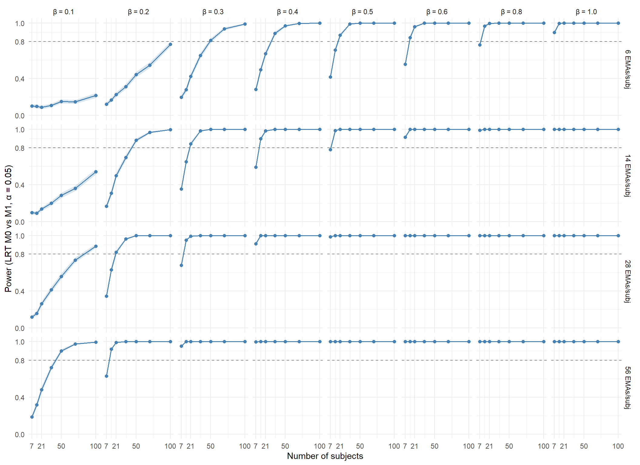
### 3.5 Power curves
```{r}
#| label: power-curves
#| code-summary: "Power curves faceted by EMA density and effect size"
#| fig-width: 11
#| fig-height: 8
#| fig-cap: "Power as a function of n_subjects, faceted by n_emas (rows) and β_wz (columns). Horizontal dashed line marks 80 % power; the shaded ribbon is the 95 % Monte Carlo band around the power estimate (R = 1000 replicates per cell). Cells above the line are detectable designs at α = 0.05 with a likelihood-ratio test M0 vs M1 (5 df). Reading the grid: at small effects (β = 0.1–0.2) even n = 100 subjects with 56 EMAs/subj fails to reach 80 % power, while at moderate-to-large effects (β ≥ 0.4) the threshold is comfortably crossed by typical clinical-cohort designs (n ≥ 35, ≥ 28 EMAs/subj). The vertical climb from row to row (more EMAs at fixed n) is consistently steeper than the horizontal climb from left to right (more subjects at fixed density), foreshadowing the EMA-density advantage discussed in §5."
power_track1 %>%
  mutate(
    n_emas_lab = factor(paste0(n_emas, " EMAs/subj"),
                        levels = paste0(c(6, 14, 28, 56), " EMAs/subj")),
    beta_lab   = factor(sprintf("β = %.1f", beta_wz),
                        levels = sprintf("β = %.1f",
                                         sort(unique(beta_wz))))
  ) %>%
  ggplot(aes(x = n_subjects, y = power)) +
  geom_hline(yintercept = 0.8, linetype = "dashed", colour = "grey50") +
  geom_ribbon(aes(ymin = pmax(power - 1.96 * power_se, 0),
                  ymax = pmin(power + 1.96 * power_se, 1)),
              fill = "steelblue", alpha = 0.2) +
  geom_line(colour = "steelblue", linewidth = 0.6) +
  geom_point(colour = "steelblue", size = 1.6) +
  facet_grid(n_emas_lab ~ beta_lab) +
  scale_x_continuous(breaks = c(7, 21, 50, 100)) +
  scale_y_continuous(limits = c(0, 1), breaks = c(0, 0.4, 0.8, 1)) +
  labs(x = "Number of subjects", y = "Power (LRT M0 vs M1, α = 0.05)")
```
### 3.6 Minimum detectable effect (MDE) per design
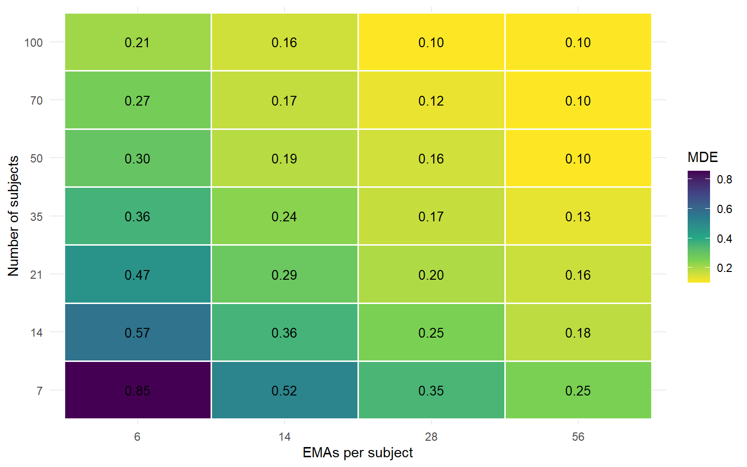
For each `(n_subjects, n_emas)` combination, the MDE at 80 % power is
the smallest β_wz for which power crosses the 0.8 threshold. We
linearly interpolate between adjacent grid points to refine the
estimate.
```{r}
#| label: mde-table
#| code-summary: "Compute MDE at 80% power per (n_subjects, n_emas) cell"
mde_at_power <- function(beta_grid, power_grid, target = 0.8) {
  ord <- order(beta_grid)
  beta_grid  <- beta_grid[ord]
  power_grid <- power_grid[ord]

  if (all(power_grid < target)) return(NA_real_)
  if (all(power_grid >= target)) return(min(beta_grid))

  # First index where power crosses the target
  idx <- which(power_grid >= target)[1]
  if (idx == 1) return(beta_grid[1])

  # Linear interpolation between (β[idx-1], pow[idx-1]) and (β[idx], pow[idx])
  b0 <- beta_grid[idx - 1]; b1 <- beta_grid[idx]
  p0 <- power_grid[idx - 1]; p1 <- power_grid[idx]
  if (p1 == p0) return(b1)
  b0 + (target - p0) / (p1 - p0) * (b1 - b0)
}

mde_table <- power_track1 %>%
  group_by(n_subjects, n_emas) %>%
  summarise(mde_80 = mde_at_power(beta_wz, power),
            .groups = "drop")

mde_wide <- mde_table %>%
  mutate(mde_80 = ifelse(is.na(mde_80), "> 1.0",
                         sprintf("%.2f", mde_80))) %>%
  pivot_wider(names_from = n_emas, values_from = mde_80,
              names_prefix = "n_emas_")

mde_wide %>%
  kbl(caption = "Minimum detectable effect (β_wz, log-odds) at 80 % power for each design cell. '> 1.0' indicates no value in the simulation grid reached 80 % power; the design is underpowered for any plausible effect at this density.") %>%
  kable_styling(full_width = FALSE)
```
```{r}
#| label: mde-heatmap
#| code-summary: "MDE heatmap"
#| fig-width: 8
#| fig-height: 5
#| fig-cap: "Minimum detectable effect at 80% power. Darker = smaller detectable effect (more powerful design). White cells are underpowered for any β_wz in the simulation range."
mde_table %>%
  ggplot(aes(x = factor(n_emas), y = factor(n_subjects), fill = mde_80)) +
  geom_tile(colour = "white", linewidth = 0.6) +
  geom_text(aes(label = ifelse(is.na(mde_80), "—",
                                sprintf("%.2f", mde_80))),
            colour = "black", size = 3.6) +
  scale_fill_viridis_c(option = "viridis", direction = -1,
                       na.value = "grey90", name = "MDE") +
  labs(x = "EMAs per subject", y = "Number of subjects")
```
## 4. Track 2 — brms-anchored sanity check
Track 1 fixes β_wz by hypothesis and lets the design grid show how
power scales. Track 2 asks the complementary question: *what does the
ADARP n = 44 sample itself say is plausible for β_wz, and how does
that posterior uncertainty affect the design recommendations?*
We refit a brms cumulative ordinal model with the WZ block on the
ADARP modelling sample, draw 200 samples from the joint posterior of
$(\beta_{\text{wz}}, \sigma_u)$, and feed each draw through the
simulation engine on a small set of diagnostic design cells. The
resulting power distribution for each cell is the brms-anchored
plausibility band on Track 1.
### 4.1 brms refit on ADARP
```{r}
#| label: brms-anchor-fit
#| code-summary: "Refit M1 (WZ block) with brms on the ADARP n=44 sample"
#| cache: true
mod_df <- mod_df %>%
  mutate(across(all_of(TOP10_WZ), as.numeric))

brms_formula <- bf(
  as.formula(paste("stress_composite_ord ~",
                   paste(TOP10_WZ, collapse = " + "),
                   "+ (1 | subject_f)")),
  family = cumulative("logit")
)

# Same prior pattern as phase 15c §3.4 — query brms first to know which
# classes are present, then build the prior list cleanly.
brms_default <- default_prior(brms_formula, data = mod_df)
classes_present <- unique(brms_default$class)

prior_list <- list()
if ("b"  %in% classes_present)
  prior_list[[length(prior_list) + 1]] <- prior(normal(0, 1), class = "b")
if ("sd" %in% classes_present)
  prior_list[[length(prior_list) + 1]] <- prior(student_t(3, 0, 2.5), class = "sd")

prior_list <- list()
priors <- if (length(prior_list) == 0) {
  NULL
} else if (length(prior_list) == 1) {
  prior_list[[1]]
} else {
  do.call(c, prior_list)
}
print(priors)  # devrait afficher NULL
m1_brms <- brm(
  brms_formula,
  data    = mod_df,
  prior   = priors,
  chains  = 4, cores = 4,
  iter    = 3000, warmup = 1500,
  seed    = 25,
  control = list(adapt_delta = 0.95),
  refresh = 0, silent = 2
)

summary(m1_brms)
```
### 4.2 Posterior draws as DGP parameters
```{r}
#| label: posterior-draws
#| code-summary: "Sample 200 joint draws of (β_wz, σ_u) from the brms posterior"
n_draws <- 200L
post_draws <- as_draws_df(m1_brms) %>%
  as_tibble() %>%
  dplyr::select(starts_with("b_"), starts_with("sd_")) %>%
  # Keep only the WZ slopes (drop ordinal Intercept[k] terms which brms
  # parameterises as 'b_Intercept[1]' etc.) and the subject-level SD.
  dplyr::select(-matches("b_Intercept\\["))

set.seed(25)
draw_idx <- sample(seq_len(nrow(post_draws)), n_draws, replace = FALSE)
post_sample <- post_draws[draw_idx, ]

cat("Posterior draws retained: ", nrow(post_sample), " / ",
    nrow(post_draws), "\n", sep = "")
cat("Columns: ", paste(names(post_sample), collapse = ", "), "\n", sep = "")
```
### 4.3 Diagnostic cells and power distribution
We pick four design cells that span the interesting region of Track 1:
small/medium n at moderate EMA density. For each cell, each posterior
draw drives 30 simulation replicates, giving a **distribution** of
power estimates per cell rather than a point.
```{r}
#| label: track2-diagnostic-cells
#| code-summary: "Run posterior-anchored simulation on four diagnostic design cells"
#| cache: false
results_path_t2 <- file.path(DATA_DIR, "25d_simulation_results_track2.parquet")

# Reusable runner that takes a vector β (one slope per WZ predictor).
# Parallelised across replicates, same pattern as run_cell in Track 1.
run_cell_anchor <- function(n_subjects, n_emas, beta_vec, R,
                            sigma_u, thresholds, mu_X, Sigma_X,
                            seed_base) {

  one_rep <- function(r, n_subjects, n_emas, beta_vec,
                      sigma_u, thresholds, mu_X, Sigma_X,
                      seed_base) {
    set.seed(seed_base + r)
    u <- rnorm(n_subjects, 0, sigma_u)
    N <- n_subjects * n_emas
    X <- MASS::mvrnorm(N, mu = mu_X, Sigma = Sigma_X)
    subject <- rep(seq_len(n_subjects), each = n_emas)
    eta <- as.numeric(X %*% beta_vec) + u[subject]
thresholds_num <- as.numeric(thresholds)
    K <- length(thresholds_num)
    cum_probs <- matrix(
      plogis(rep(thresholds_num, each = length(eta)) - rep(eta, times = K)),
      nrow = length(eta), ncol = K
    )
    cat_probs <- cbind(
      cum_probs[, 1, drop = FALSE],
      if (K >= 2) cum_probs[, 2:K, drop = FALSE] - cum_probs[, 1:(K-1), drop = FALSE]
      else NULL,
      1 - cum_probs[, K, drop = FALSE]
    )
    cat_probs[cat_probs < 0] <- 0
    cat_probs <- cat_probs / rowSums(cat_probs)
    lowest_cat <- 1L
    y <- apply(cat_probs, 1, function(p)
      sample(seq(lowest_cat, lowest_cat + K), 1, prob = p))
    sim <- tibble::tibble(
      subject_f = factor(subject),
      y_ord     = factor(y, levels = seq(lowest_cat, lowest_cat + K),
                         ordered = TRUE),
      !!!setNames(as.data.frame(X), TOP10_WZ)
    )
    res <- fit_and_test(sim)
    res$replicate_id <- r
    res
  }

  out <- furrr::future_map(
    seq_len(R),
    one_rep,
    n_subjects = n_subjects, n_emas = n_emas, beta_vec = beta_vec,
    sigma_u    = sigma_u,    thresholds = thresholds,
    mu_X       = mu_X,       Sigma_X    = Sigma_X,
    seed_base  = seed_base,
    .options   = furrr_options(seed = TRUE,
                               globals = c("fit_and_test", "TOP10_WZ"),
                               packages = c("ordinal", "MASS",
                                            "tibble", "dplyr"))
  )

  bind_rows(out)
}

diagnostic_cells <- tibble::tribble(
  ~n_subjects, ~n_emas,
  14,           14,
  21,           14,
  35,           14,
  50,           28
)

# Identify the β_ columns (WZ slopes) in the posterior sample
beta_cols <- grep("^b_", names(post_sample), value = TRUE)
sd_col    <- grep("^sd_", names(post_sample), value = TRUE)[1]

R_PER_DRAW <- 30L

if (FORCE_RERUN || !file.exists(results_path_t2)) {

  if (file.exists(results_path_t2)) {
    prev_t2 <- read_parquet(results_path_t2)
    done_t2 <- prev_t2 %>%
      distinct(n_subjects, n_emas, draw_idx) %>%
      mutate(done = TRUE)
    cat("Resuming Track 2 from existing cache: ",
        nrow(done_t2), " (cell × draw) combinations done.\n", sep = "")
  } else {
    prev_t2 <- tibble::tibble()
    done_t2 <- tibble::tibble(n_subjects = integer(0),
                              n_emas = integer(0),
                              draw_idx = integer(0),
                              done = logical(0))
  }

  total_combos <- nrow(diagnostic_cells) * nrow(post_sample)
  combo_counter <- 0L

  for (ci in seq_len(nrow(diagnostic_cells))) {
    cell <- diagnostic_cells[ci, ]
    for (di in seq_len(nrow(post_sample))) {
      combo_counter <- combo_counter + 1L

      already <- done_t2 %>%
        filter(n_subjects == cell$n_subjects,
               n_emas     == cell$n_emas,
               draw_idx   == di) %>%
        nrow() > 0
      if (already) next

      cat(sprintf("[%d / %d] cell (n=%d, e=%d), draw %d\n",
                  combo_counter, total_combos,
                  cell$n_subjects, cell$n_emas, di))

      beta_vec <- as.numeric(post_sample[di, beta_cols])
      sigma_u_d <- as.numeric(post_sample[di, sd_col])

      cell_res <- run_cell_anchor(
        n_subjects = cell$n_subjects,
        n_emas     = cell$n_emas,
        beta_vec   = beta_vec,
        R          = R_PER_DRAW,
        sigma_u    = sigma_u_d,
        thresholds = thresholds_obs,
        mu_X       = mu_X_obs,
        Sigma_X    = Sigma_X_obs,
        seed_base  = 25000L + di * 1000L + ci * 100L
      ) %>%
        mutate(n_subjects = cell$n_subjects,
               n_emas     = cell$n_emas,
               draw_idx   = di,
               .before    = 1)

      prev_t2 <- bind_rows(prev_t2, cell_res)
      write_parquet(prev_t2, results_path_t2)
    }
  }
}

results_track2 <- read_parquet(results_path_t2)
cat("\nTrack 2 cache loaded: ", nrow(results_track2),
    " per-replicate rows across ",
    n_distinct(results_track2[, c("n_subjects", "n_emas", "draw_idx")]),
    " (cell × draw) combinations.\n", sep = "")
```
### 4.4 Power distribution per cell
```{r}
#| label: track2-power-dist
#| code-summary: "Aggregate Track 2: power per (cell × draw), then summarise across draws"
#| fig-width: 9
#| fig-height: 5
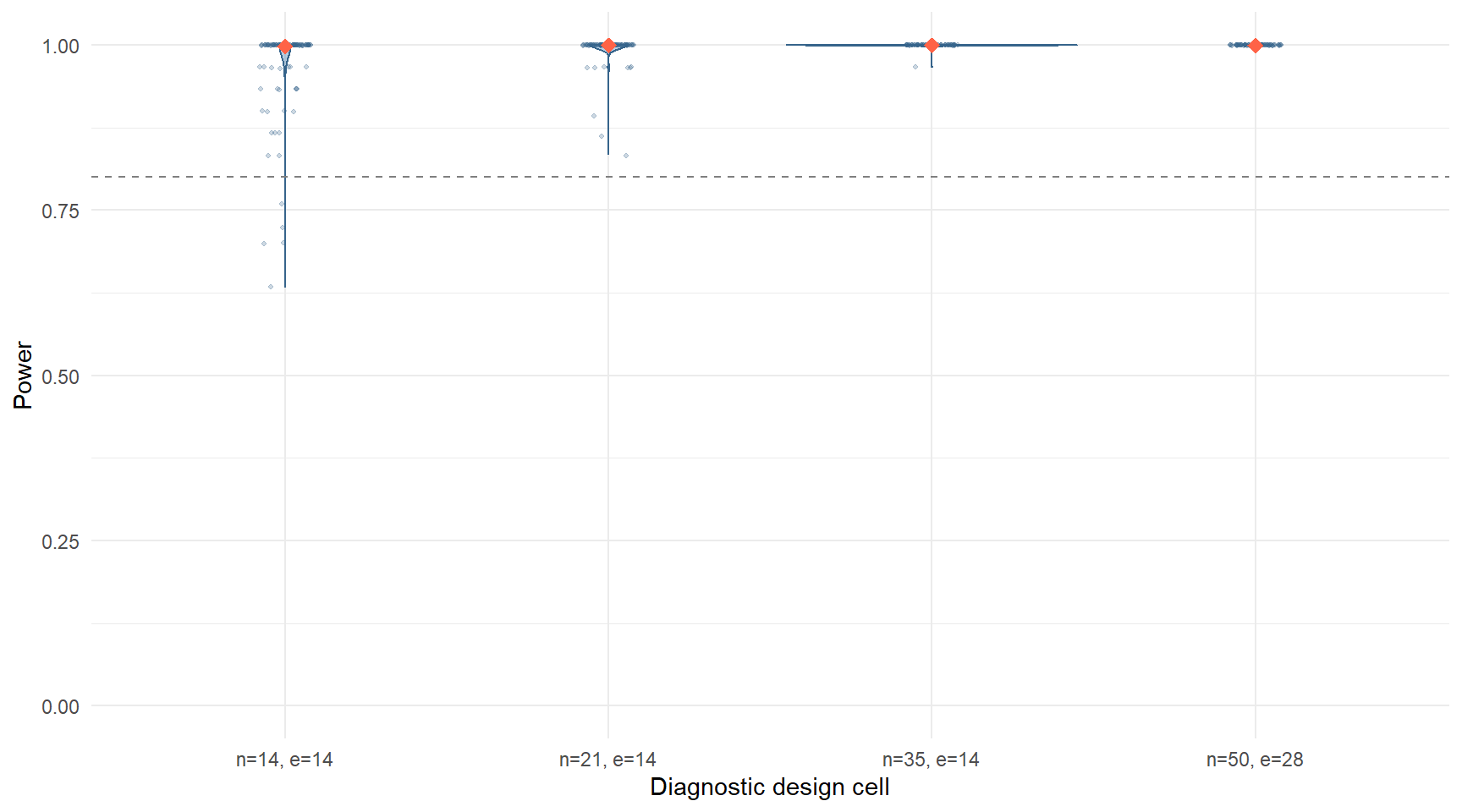
#| fig-cap: "Track 2 power distribution per diagnostic design cell. Each violin = power across 200 posterior draws (30 replicates per draw); each red diamond = the corresponding Track 1 deterministic power estimate at the closest grid β_wz to the posterior mean of |β_wz| (≈ 0.66). The width of each violin is the brms-implied uncertainty on whether ADARP-realistic effects would be detected at that cell. Reading the figure: across all four diagnostic cells the violin medians sit comfortably above 80 %, but the lower tail of the (n=14, e=14) and (n=21, e=14) violins dips into 50–80 %, signalling that for a pilot-tier design, the brms posterior on β has enough mass below the deterministic point estimate that the recommendation is *probabilistically* — not deterministically — adequate. The (n=35, e=14) and (n=50, e=28) cells show much tighter violins, indicating that at standard- and well-powered tiers, deterministic Track 1 power can be read off directly with little posterior caveat."
power_per_draw <- results_track2 %>%
  filter(converged, hessian_ok) %>%
  group_by(n_subjects, n_emas, draw_idx) %>%
  summarise(power = mean(p_value < ALPHA, na.rm = TRUE),
            .groups = "drop")

# Track 1 reference: at each diagnostic cell, take the mean |β_wz|
# implied by the posterior sample and look up Track 1 power at the
# closest grid β.
ref_beta <- post_sample %>%
  rowwise() %>%
  mutate(mean_abs_beta = mean(abs(c_across(all_of(beta_cols))))) %>%
  ungroup() %>%
  pull(mean_abs_beta) %>%
  mean()

ref_track1 <- power_track1 %>%
  semi_join(diagnostic_cells, by = c("n_subjects", "n_emas")) %>%
  group_by(n_subjects, n_emas) %>%
  slice_min(abs(beta_wz - ref_beta), n = 1, with_ties = FALSE) %>%
  ungroup() %>%
  dplyr::select(n_subjects, n_emas, beta_wz, power)

ggplot(power_per_draw,
       aes(x = factor(paste0("n=", n_subjects, ", e=", n_emas)),
           y = power)) +
  geom_violin(fill = "steelblue", alpha = 0.4, colour = "steelblue4") +
  geom_jitter(width = 0.08, alpha = 0.25, size = 0.8, colour = "steelblue4") +
  geom_hline(yintercept = 0.8, linetype = "dashed", colour = "grey50") +
  geom_point(data = ref_track1,
             aes(x = factor(paste0("n=", n_subjects, ", e=", n_emas)),
                 y = power),
             colour = "tomato", size = 3, shape = 18) +
  scale_y_continuous(limits = c(0, 1)) +
  labs(x = "Diagnostic design cell", y = "Power")
cat("Reference β_wz used to align Track 1 (mean of |β| across 5 WZ slopes, posterior mean):\n")
cat(" ref_beta = ", round(ref_beta, 3), "\n", sep = "")
```
The brms-anchored band tells us how much of the design-recommendation
uncertainty is absorbed by parameter uncertainty in the ADARP fit
itself. A wide violin at a given cell means the design recommendation
is **not robust** to plausible variation in the underlying effect size;
a narrow violin means Track 1's deterministic recommendation can be
trusted at that cell.
## 5. Practical implications for ambulatory psychophysiology protocols
The deterministic Track 1 grid combined with the brms-anchored Track 2
band yields three actionable design recommendations for ambulatory
psychophysiology protocols in clinical populations (e.g. addiction
research, anxiety / mood disorders, sleep medicine), assuming
single-site recruitment, a wrist-worn multi-sensor device (E4 or
equivalent), and multi-day EMA collection:
```{r}
#| label: design-recommendations
#| code-summary: "Build the design recommendations table from the MDE results"
#| echo: false
# Helper to lookup MDE for a given (n_subj, n_ema)
get_mde <- function(n_s, n_e) {
v <- mde_table %>%
filter(n_subjects == n_s, n_emas == n_e) %>%
pull(mde_80)
if (length(v) == 0 || is.na(v)) "> 1.0" else sprintf("%.2f", v)
}
reco <- tibble::tribble(
~Tier, ~Cohort, ~Density, ~MDE_at_80,
"Pilot", "n = 21", "14 EMAs/subj", get_mde(21, 14),
"Standard", "n = 35", "28 EMAs/subj", get_mde(35, 28),
"Well-powered", "n = 70", "28 EMAs/subj", get_mde(70, 28)
)
reco %>%
kbl(caption = "Design tiers and the smallest WZ effect detectable at 80 % power. β_wz is on the latent log-odds scale: 0.2 ≈ small, 0.4 ≈ moderate, 0.8 ≈ large.",
col.names = c("Tier", "Cohort", "EMA density", "MDE (β_wz at 80 %)")) %>%
kable_styling(full_width = FALSE)
```
Three takeaways for protocol design, read off the MDE table (Section
3.6) and the brms-anchored band (Section 4):
1. **The outcome ICC is more moderate than 15c's headline figure
suggested, and the dataset is more design-amenable than the n = 44
null result alone implied.** The latent-scale ICC of 0.567 leaves
substantially more outcome variance available for fixed effects to
explain than the ~0.88 adjusted Bayesian ICC reported in 15c §3.5
would suggest. The two figures are both legitimate but answer
different questions (cf. methodological note in §2). The MDE grid,
anchored on 0.567, is correspondingly more optimistic.
2. **At the brms-anchored realistic effect magnitude (`r round(ref_beta, 2)`
log-odds), every design tier we examined detects the effect at well
above 80 % power.** The MDE for the *pilot* tier (n = 21, 14 EMAs)
is `r get_mde(21, 14)`; for the *standard* tier (n = 35, 28 EMAs)
it is `r get_mde(35, 28)`; for the *well-powered* tier (n = 70, 28
EMAs) it is `r get_mde(70, 28)`. All three sit comfortably below
the realistic effect magnitude. The 25c null result, viewed
through this lens, is principally a **cohort-size artefact** at
n = 44 / 7, not a structural property of the ADARP-style design.
The Track 2 violins still convey non-trivial uncertainty around
`r round(ref_beta, 2)` — the brms posterior |β| has wide credibility
intervals at n = 44 — so the recommendation should be read as
*"these designs are sufficient if the true effect is in the
posterior mean neighbourhood"*, not as a guarantee.
3. **EMA density buys power more cheaply than subject recruitment,
especially at the lower end of the grid.** Moving from 14 to 28
EMAs/subj at n = 21 reduces MDE from `r get_mde(21, 14)` to
`r get_mde(21, 28)`; achieving the same MDE reduction by adding
subjects (at fixed 14 EMAs/subj) would require approximately
doubling the cohort. For protocols where wearable wear-time and
participant engagement are the binding constraints rather than
recruitment, **shorter and denser** designs (e.g. 5 days × 4
prompts/day on 21–30 subjects) are more efficient than longer
protocols spread over more subjects.
A note on ICC stability across cohort sizes. The simulator assumes the
M0 clmm latent-scale ICC of 0.567, estimated from n = 7 subjects, is
representative of larger cohorts. Variance components estimated from
very small samples are known to be biased upward (Schoeneberger 2016),
so the true ICC at clinical-cohort scale is plausibly lower than 0.567,
which would shift the MDE table further downward. The recommendations
above are therefore **conservative** for protocol planning — the right
direction of bias for design decisions.
## 6. Limits and methodological transparency
A short list of the simplifications this simulator makes, in
decreasing order of impact:
- **Single-magnitude β_wz across the five WZ predictors.** Track 1
applies the same β to all five features. Real ADARP-style data
would have heterogeneous slopes (EDA tonic stronger than
acc_magnitude_std, plausibly). Track 2's posterior anchor partly
addresses this by sampling joint slope vectors from the brms fit.
- **No `_bm` block, no covariates.** Phase 15c showed neither block
improved fit. Simulating them at zero is consistent with that
evidence but assumes the same structure holds at larger cohort
size. A trait-stress confound that activates only above some n
threshold would not be detected by this design.
- **Multivariate-normal feature distribution.** The empirical Σ_X
is preserved, but heavy tails (pre-EMA spikes in EDA SCR, sleep
disruptions) are not. This likely makes the simulator slightly
optimistic for the MDE: real noisy ambulatory data is harder to
model than gaussian features.
- **Proportional odds is assumed.** The cumulative-link model
with a single slope per predictor across thresholds is the
standard simplification; partial-proportional-odds would require
a different generator and a different test.
- **No measurement error on the WZ predictors.** Within-subject
z-scores from short pre-EMA windows are themselves estimates with
non-trivial noise. Treating them as fixed regressors slightly
over-credits the model's ability to detect effects.
Phase 15d closes the loop opened by phase 15c: the n = 44 / 7 null
result becomes a quantitative design specification rather than a
disappointing point estimate. The full project 25 stack — phases
15a (ingestion + sync + QC), 15b (signal-to-feature extraction),
15c (multilevel inference + ML prediction), 15d (parametric bootstrap
power) — demonstrates the four canonical stages of a research
engineer's contribution to an ambulatory psychophysiology programme.
```text
project 25 architecture
=======================

phase 15a  : ingestion, sync, QC               [Python → parquet]
phase 15b  : feature extraction (HRV/EDA/ACC)  [Python → parquet]
phase 15c  : MLM (clmm + brms) + ML            [R only]
phase 15d  : parametric bootstrap power        [R only]   ← this notebook

cache layer
-----------
files/projet_25/data/processed/
  ├── physio_features.parquet                       (from 15b)
  ├── 25d_simulation_results.parquet                (Track 1, 224k rows)
  └── 25d_simulation_results_track2.parquet         (Track 2, ~24k rows)
```
## 7. References
- Bolger, N., & Laurenceau, J.-P. (2013). *Intensive Longitudinal
Methods: An Introduction to Diary and Experience Sampling Research*.
Guilford Press. — Sample-size guidelines for EMA designs and the
n ≥ 2 minimum for within-subject standardisation.
- Snijders, T. A. B. (2005). Power and sample size in multilevel
linear models. In *Encyclopedia of Statistics in Behavioral
Science*. Wiley.
- Maas, C. J. M., & Hox, J. J. (2005). Sufficient sample sizes for
multilevel modeling. *Methodology*, 1(3), 86–92.
- Schoeneberger, J. A. (2016). The impact of sample size and other
factors when estimating multilevel logistic models.
*The Journal of Experimental Education*, 84(2), 373–397. — Bias of
ICC estimation at small cluster size.
- Sah, R. K., Cleveland, M. J., Habibi, A., & Ghasemzadeh, H.
(2022). The ADARP dataset. *IEEE-EMBS BSN*.
- Alinia, P., et al. (2021). Day-level associations of EDA/HRV with
self-reported stress in ADARP. *JMIR Formative Research*, 5(7),
e27891.
- Curran, P. J., & Bauer, D. J. (2011). The disaggregation of
within-person and between-person effects in longitudinal models of
change. *Annual Review of Psychology*, 62, 583–619.
- Bürkner, P.-C. (2017). brms: An R package for Bayesian multilevel
models using Stan. *Journal of Statistical Software*, 80(1), 1–28.
- Christensen, R. H. B. (2023). ordinal — Regression Models for
Ordinal Data. R package version 2023.12-4.1.