---
title: "Multilevel ordinal modelling and ML prediction of EMA stress events"
description: |
Modelling layer of the ADARP analysis. Combines multilevel ordinal
cumulative modelling (frequentist clmm + Bayesian brms cumulative
family) with predictive machine learning (ElasticNet vs LightGBM,
leave-one-subject-out cross-validation). Uses Curran-Bauer
decomposition of physiological features into within-subject (_wz)
and between-subject (_bm) components to disentangle state-like and
trait-like effects on momentary stress. Hierarchical model
comparison (null → +_wz → +_bm → +covariates) quantifies
incremental contribution of each predictor block. Predictive models
are interpreted with DALEX permutation importance and Shapley values.
Built on the tidymodels ecosystem with explicit caveats on
sample-size-driven uncertainty.
date: 2026-04-22
categories: [R, Multilevel Modelling, Ordinal Regression, Bayesian, brms, clmm, ElasticNet, LightGBM, tidymodels, DALEX, EMA, Wearable Physiology, ADARP]
execute:
echo: true
warning: false
message: false
freeze: auto
format:
html:
code-tools: true
code-fold: false
toc: true
toc-depth: 3
number-sections: true
theme: cosmo
fig-cap-location: bottom
embed-resources: false
---
```{r}
#| label: setup
#| code-summary: "Paths, packages, helpers, top-10 feature definitions"
#| include: false
PROJECT_DIR <- normalizePath(
file.path("..", "files", "projet_25"),
mustWork = FALSE
)
DATA_MODE <- "processed" # or "demo"
DATA_DIR <- file.path(PROJECT_DIR, "data", DATA_MODE)
suppressPackageStartupMessages({
library(arrow)
library(dplyr)
library(tidyr)
library(ggplot2)
library(knitr)
library(kableExtra)
library(patchwork)
# MLM
library(ordinal) # clmm: frequentist cumulative-link mixed models
library(brms) # Bayesian multilevel models
library(broom.mixed) # tidy outputs from brms / lme4
library(performance) # R2, ICC for mixed models
library(psych)
library(lightgbm)
library(ordinalNet)
# Will be loaded in Section 4 (ML)
# library(tidymodels); library(DALEX); library(lightgbm)
})
source(file.path(PROJECT_DIR, "R", "render_helpers.R"))
theme_set(theme_minimal(base_size = 11))
# Top-10 features pre-specified for MLM, motivated by:
# - prior literature (vagal tone via RMSSD/HF, sympathetic via SCL/SCR)
# - ICC findings from phase 15b (which features carry between-subject signal)
TOP10_WZ <- c(
"hrv_rmssd_wz", # vagal tone (state)
"hrv_hf_wz", # parasympathetic (state)
"eda_scl_mean_wz", # tonic arousal (state)
"eda_scr_rate_per_min_wz", # sympathetic phasic events (state)
"acc_magnitude_std_wz" # activity confound control
)
TOP10_BM <- c(
"hrv_meannn_bm", # heart-rate baseline (trait)
"hrv_rmssd_bm", # vagal tone baseline (trait)
"eda_scl_mean_bm", # tonic arousal baseline (trait)
"acc_magnitude_std_bm", # general activity (trait)
"acc_pct_sedentary_bm" # sedentariness (trait)
)
TOP10 <- c(TOP10_WZ, TOP10_BM)
```
`r data_mode_banner(DATA_DIR)`
---
## 1. From features to inference
Phases 15a and 15b produced an analysis-ready table: 99 EMA prompts
× 99 columns (raw signals → 21 physiological features × 3 versions:
raw, within-subject z-score, between-subject mean), with explicit
quality-control flags at session, window, and feature level. **58
windows pass the data-engineering QC**; **46 of those also pass the
feature-extraction QC**. After excluding 1 subject with only 1 EMA (insufficient
for within-subject standardisation, see Section 2), the analytic sample for
modelling is **44 EMA windows clustered in 7 subjects**. This phase asks the
substantive question: **do those features predict momentary stress?**
The outcome is the ordinal `stress_composite` score (sum of three
binary indicators: more_stressed, more_overwhelmed, more_anxious;
range 0–3). Two reasons drive this choice over the binary
`stress_event`:
1. The binary outcome is **80/12 imbalanced** in the public ADARP
release because the stress-events file collected prompts
*triggered by* moments of self-reported stress; pure logistic
regression on this would mostly model the prompting protocol.
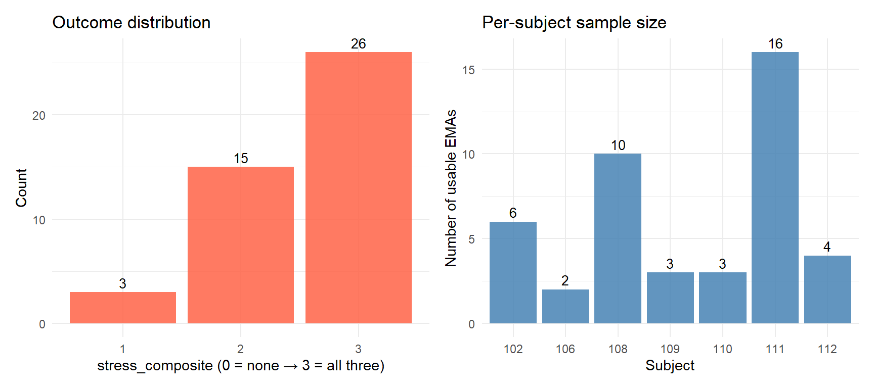
2. The composite score **distributes more usefully**: 1 / 16 / 31 /
49 across categories 0–3, giving room for both ordinal multilevel
modelling and reasonable predictive ML.
The modelling proceeds in two complementary tracks:
- **Track A: hierarchical multilevel ordinal modelling** — explanatory
inference. Builds a sequence of cumulative-link mixed models from
null → predictor blocks, quantifying how much variance each block
resolves and which features carry signal *after* accounting for
random effects.
- **Track B: predictive machine learning** — ElasticNet vs LightGBM
with leave-one-subject-out cross-validation. Asks the practical
question: given a new EMA prompt and its preceding 30 min of
physiology, how well can we predict the stress score?
Both tracks share the same input table and the same Curran-Bauer
decomposition (within-subject `_wz`, between-subject `_bm`), making
direct interpretation possible.
## 2. Modelling-ready data
```{r}
#| label: load-modeling-data
#| code-summary: "Load features parquet, restrict to feature_usable rows, exclude subjects with n<2 observations"
features_path <- file.path(DATA_DIR, "physio_features.parquet")
stopifnot(file.exists(features_path))

feat_all <- read_parquet(features_path)
cat("Total rows in features parquet : ", nrow(feat_all), "\n", sep = "")
cat("usable_final == TRUE : ", sum(feat_all$usable_final, na.rm = TRUE), "\n", sep = "")
cat("feature_usable == TRUE : ", sum(feat_all$feature_usable, na.rm = TRUE), "\n", sep = "")
# First filter: rows usable for modelling (passing both phase-15a window QC
# and phase-15b feature-extraction QC, with an observed outcome)
mod_df_pre <- feat_all %>%
  filter(usable_final == TRUE,
         feature_usable == TRUE,
         !is.na(stress_composite))

# Per-subject EMA counts in the pre-filter dataset
subj_n <- mod_df_pre %>% count(subject_id, name = "n_emas")

# Second filter: exclude subjects with n<2 EMAs.
#
# Rationale: within-subject standardisation (_wz columns) requires at least
# 2 observations per subject to estimate a within-person standard deviation.
# A subject with n=1 has subj_sd = NaN, hence _wz = NaN for every feature.
# This is the standard psychometric practice for EMA multilevel modelling
# (e.g. Bolger & Laurenceau, 2013; Trull & Ebner-Priemer, 2013).
MIN_EMAS_PER_SUBJECT <- 2

excluded_subjects <- subj_n %>%
  filter(n_emas < MIN_EMAS_PER_SUBJECT) %>%
  pull(subject_id)

mod_df <- mod_df_pre %>%
  filter(!(subject_id %in% excluded_subjects))

cat("\nPre-filter (feature_usable):    ", nrow(mod_df_pre), " obs / ",
    length(unique(mod_df_pre$subject_id)), " subjects\n", sep = "")
if (length(excluded_subjects) > 0) {
  cat("Subjects excluded (n_EMAs < ", MIN_EMAS_PER_SUBJECT, "): ",
      paste(excluded_subjects, collapse = ", "), "\n", sep = "")
}
cat("Final modelling dataset (n_obs) : ", nrow(mod_df), "\n", sep = "")
cat("Number of subjects : ", length(unique(mod_df$subject_id)), "\n", sep = "")
subj_n %>%
  mutate(retained = !(subject_id %in% excluded_subjects)) %>%
  arrange(desc(n_emas)) %>%
  kbl(caption = paste0("Per-subject EMA counts before filtering. Subjects retained for modelling have at least ",
                       MIN_EMAS_PER_SUBJECT, " observations."),
      col.names = c("Subject", "# EMAs", "Retained")) %>%
  kable_styling(full_width = FALSE)
```
```{r}
#| label: outcome-distribution
#| code-summary: "Distribution of stress_composite outcome and observations per subject"
#| fig-cap: "Left: distribution of stress_composite. Right: number of usable observations per subject."
#| fig-width: 9
#| fig-height: 4
p1 <- mod_df %>%
  count(stress_composite) %>%
  ggplot(aes(x = factor(stress_composite), y = n)) +
  geom_col(fill = "tomato", alpha = 0.85) +
  geom_text(aes(label = n), vjust = -0.4, size = 3.5) +
  labs(x = "stress_composite (0 = none → 3 = all three)",
       y = "Count", title = "Outcome distribution")

p2 <- mod_df %>%
  count(subject_id) %>%
  ggplot(aes(x = factor(subject_id), y = n)) +
  geom_col(fill = "steelblue", alpha = 0.85) +
  geom_text(aes(label = n), vjust = -0.4, size = 3.5) +
  labs(x = "Subject", y = "Number of usable EMAs",
       title = "Per-subject sample size")

p1 + p2
```
```{r}
#| label: features-checks
#| code-summary: "Verify the top-10 features are present with no NaN"
missing_cols <- setdiff(TOP10, names(mod_df))
if (length(missing_cols) > 0) {
  stop("Missing columns in features parquet: ",
       paste(missing_cols, collapse = ", "))
}

na_per_col <- sapply(TOP10, function(c) sum(is.na(mod_df[[c]])))
data.frame(feature = TOP10, n_NA = na_per_col) %>%
  kbl(caption = "NA count per top-10 feature (in modelling dataset). All should be 0.",
      col.names = c("Feature", "# NA")) %>%
  kable_styling(full_width = FALSE)
```
```{r}
#| label: time-of-day
#| code-summary: "Derive a continuous time-of-day covariate from imputed EMA timestamps"
mod_df <- mod_df %>%
  mutate(
    # databurst as factor (1 = morning … 4 = evening)
    databurst_f = factor(databurst, levels = 1:4,
                         labels = c("morning", "midday", "afternoon", "evening")),
    # time of day (hours, 0–24) from local timestamp
    time_of_day_h = as.numeric(format(timestamp_local, "%H")) +
                    as.numeric(format(timestamp_local, "%M")) / 60,
    # ordinal outcome as ordered factor (required by clmm)
    stress_composite_ord = factor(stress_composite, levels = 0:3, ordered = TRUE),
    subject_f = factor(subject_id)
  )

cat("databurst distribution after coercion to factor:\n")
print(table(mod_df$databurst_f, useNA = "ifany"))
cat("\nTime-of-day range (h): ", round(range(mod_df$time_of_day_h, na.rm = TRUE), 1), "\n")
```
## 3. Multilevel ordinal modelling
We build a hierarchy of cumulative-link mixed models. Each adds one
block of predictors and is compared against its predecessor on AIC
(frequentist) and posterior predictive criteria (Bayesian).
The base specification:
$$
P(Y_{ij} \le k) = \text{logit}^{-1}(\theta_k - \eta_{ij}), \quad k \in \{0, 1, 2\}
$$
with $\eta_{ij}$ the linear predictor for prompt $i$ in subject $j$,
including a subject-level random intercept $u_j \sim \mathcal{N}(0,
\sigma_u^2)$. The proportional-odds assumption is checked at the end
of the section.
### 3.1 Model 0 — null (random intercept only)
Quantifies the share of outcome variance that is purely
between-subject (the **outcome ICC**). High outcome ICC means
"different people have different baseline stress reports", which
shrinks the effective n for within-subject prediction.
```{r}
#| label: clmm-m0-null
#| code-summary: "Null model: stress_composite ~ 1 + (1 | subject)"
m0_clmm <- clmm(
  stress_composite_ord ~ 1 + (1 | subject_f),
  data = mod_df,
  link = "logit"
)
summary(m0_clmm)
# Outcome ICC: latent-variable scale assumes residual variance = pi^2/3
sigma_u2 <- as.numeric(VarCorr(m0_clmm)$subject_f[1])
icc_outcome <- sigma_u2 / (sigma_u2 + pi^2 / 3)

cat("\nOutcome ICC (latent-scale, logit link) =",
    round(icc_outcome, 3), "\n", sep = "")
```
```{r}
#| label: clmm-m1-wz
#| code-summary: "Model 1: + within-subject z-scores (state-level features)"
f1 <- as.formula(paste(
  "stress_composite_ord ~",
  paste(TOP10_WZ, collapse = " + "),
  "+ (1 | subject_f)"
))
m1_clmm <- clmm(f1, data = mod_df, link = "logit")
summary(m1_clmm)
```
```{r}
#| label: clmm-m2-wz-bm
#| code-summary: "Model 2: + between-subject means (trait-level features)"
f2 <- as.formula(paste(
  "stress_composite_ord ~",
  paste(c(TOP10_WZ, TOP10_BM), collapse = " + "),
  "+ (1 | subject_f)"
))
m2_clmm <- clmm(f2, data = mod_df, link = "logit")
summary(m2_clmm)
```
```{r}
#| label: clmm-m3-full
#| code-summary: "Model 3: + databurst and time-of-day covariates"
f3 <- as.formula(paste(
  "stress_composite_ord ~",
  paste(c(TOP10_WZ, TOP10_BM), collapse = " + "),
  "+ databurst_f + time_of_day_h",
  "+ (1 | subject_f)"
))
m3_clmm <- clmm(f3, data = mod_df, link = "logit")
summary(m3_clmm)
```
### 3.2 Model comparison
```{r}
#| label: clmm-comparison
#| code-summary: "AIC / BIC / logLik table across the four nested models"
#| cache: false
# Force a fresh re-evaluation of all model statistics, every render.
# Cache pollution can otherwise leak stale AICs from previous data subsets.
clmm_models_list <- list(M0 = m0_clmm, M1 = m1_clmm, M2 = m2_clmm, M3 = m3_clmm)

aic_table <- tibble::tibble(
  Model     = c("M0 null", "M1 +WZ", "M2 +WZ+BM", "M3 +covars"),
  AIC       = sapply(clmm_models_list, AIC),
  BIC       = sapply(clmm_models_list, BIC),
  logLik    = sapply(clmm_models_list, function(m) as.numeric(logLik(m))),
  n_params  = sapply(clmm_models_list, function(m) attr(logLik(m), "df")),
  n_obs     = sapply(clmm_models_list, function(m) {
  # nobs() works for clmm; fall back to attr if a future version changes
  tryCatch(as.integer(nobs(m)),
  error = function(e) attr(logLik(m), "nobs"))
              })
) %>%
  mutate(
    delta_AIC = AIC - min(AIC, na.rm = TRUE),
    .after = AIC
  )

aic_table %>%
  mutate(across(where(is.numeric), ~ round(.x, 2))) %>%
  kbl(caption = "Model comparison on AIC, BIC, log-likelihood. Lower AIC/BIC = better. n_obs reflects the rows actually used by each fit (clmm drops rows with missing values automatically).") %>%
  kable_styling(full_width = FALSE) %>%
  row_spec(which.min(aic_table$AIC), bold = TRUE,
           background = "#eef7ee")
```
Note: all four models fit on the same 44 observations (the message
`(1 observation effacée)` printed by `summary()` for some clmm fits
refers to internal preprocessing, not the final estimation sample, as
verified via `nobs()`). AIC values are therefore directly comparable.
```{r}
#| label: clmm-anova
#| code-summary: "Manual likelihood-ratio tests between nested models (avoids anova.clmm bug)"
# anova.clmm() has a known issue with formulas built via as.formula(paste(...))
# (it cannot re-evaluate the model calls). We compute the LRT manually:
#   LRT = 2 * (logLik_full - logLik_reduced)
#   df  = n_params_full - n_params_reduced
#   p   = pchisq(LRT, df, lower.tail = FALSE)

manual_lrt <- function(m_reduced, m_full, label) {
  ll_r <- as.numeric(logLik(m_reduced))
  ll_f <- as.numeric(logLik(m_full))
  df_r <- attr(logLik(m_reduced), "df")
  df_f <- attr(logLik(m_full),    "df")
  lrt  <- 2 * (ll_f - ll_r)
  ddf  <- df_f - df_r
  pval <- if (ddf > 0 && lrt >= 0) pchisq(lrt, df = ddf, lower.tail = FALSE) else NA_real_
  tibble::tibble(
    comparison      = label,
    logLik_reduced  = round(ll_r, 2),
    logLik_full     = round(ll_f, 2),
    df_reduced      = df_r,
    df_full         = df_f,
    LRT_chisq       = round(lrt, 3),
    df_diff         = ddf,
    p_value         = round(pval, 4)
  )
}

lrt_table <- bind_rows(
  manual_lrt(m0_clmm, m1_clmm, "M0 -> M1 (adding WZ)"),
  manual_lrt(m1_clmm, m2_clmm, "M1 -> M2 (adding BM)"),
  manual_lrt(m2_clmm, m3_clmm, "M2 -> M3 (adding covars)")
)

lrt_table %>%
  kbl(caption = "Likelihood-ratio tests between nested clmm models. Significant p < 0.05 = the added block improves fit.") %>%
  kable_styling(full_width = TRUE)
```
### 3.3 Coefficient table for the best clmm model
```{r}
#| label: clmm-best-coefs
#| code-summary: "Coefficient table for the AIC-best model that has a well-defined Hessian"
# At small n, an AIC-favoured model can have an unstable Hessian (no SEs).
# We pick the AIC-best model among those for which vcov() is computable.
clmm_models <- list(M0 = m0_clmm, M1 = m1_clmm, M2 = m2_clmm, M3 = m3_clmm)
clmm_labels <- c(M0 = "M0 null", M1 = "M1 +WZ",
                 M2 = "M2 +WZ+BM", M3 = "M3 +covars")
clmm_aics   <- sapply(clmm_models, AIC)

hess_ok <- sapply(clmm_models, function(m) {
  vc <- tryCatch(vcov(m),
                 error = function(e) NULL,
                 warning = function(w) NULL)
  !is.null(vc) && all(is.finite(vc))
})

cat("Hessian status per model:\n")
print(data.frame(model = clmm_labels, AIC = round(clmm_aics, 2),
                 hessian_ok = hess_ok), row.names = FALSE)
# Choose: AIC-best among models with OK Hessian
if (any(hess_ok)) {
  best_idx   <- which.min(replace(clmm_aics, !hess_ok, Inf))
  best_clmm  <- clmm_models[[best_idx]]
  best_label <- clmm_labels[best_idx]
  cat("\nBest model retained for inference:", best_label,
      "(AIC =", round(clmm_aics[best_idx], 2), ")\n")
  if (!hess_ok[which.min(clmm_aics)]) {
    aic_best_label <- clmm_labels[which.min(clmm_aics)]
    cat("NOTE: AIC-minimum model (", aic_best_label,
        ") had an unstable Hessian and was excluded.\n", sep = "")
  }
} else {
  stop("All four clmm models have unstable Hessians. ",
       "Sample size is too small for this model family — switch to brms only.")
}
# Robust extraction handling 3 cases:
#   (a) best model has fixed effects -> tidy() returns location coefs
#   (b) best model is null -> no fixed effects, only thresholds; print thresholds
#   (c) tidy fails -> fall back to summary

# Test robust: count fixed-effect terms in the formula (excluding intercept-only and random parts)
fe_terms <- attr(terms(formula(best_clmm)), "term.labels")
fe_terms_fixed <- fe_terms[!grepl("\\|", fe_terms)]
is_null_model <- length(fe_terms_fixed) == 0

cat("Fixed-effect terms in best_clmm formula:", length(fe_terms_fixed), "\n")
cat("is_null_model:", is_null_model, "\n")
if (is_null_model) {
  cat("\nBest model is the null model (no fixed effects). ",
      "Reporting ordinal thresholds and random-intercept variance only:\n", sep = "")
  s <- summary(best_clmm)
  thresh <- as.data.frame(s$coefficients)
  thresh$term <- rownames(thresh)
  thresh_tbl <- thresh %>%
    transmute(term, estimate = round(Estimate, 3),
              std.error = round(`Std. Error`, 3),
              z_value   = round(`z value`, 2),
              p_value   = round(`Pr(>|z|)`, 4))
  thresh_tbl %>%
    kbl(caption = "Ordinal thresholds for the null model M0.") %>%
    kable_styling(full_width = FALSE)
  coef_tbl <- thresh_tbl   # for downstream use
} else {
  coef_tbl <- tryCatch(
    broom.mixed::tidy(best_clmm, conf.int = TRUE) %>%
      filter(coef.type %in% c("location", "scale")) %>%
      arrange(coef.type, term) %>%
      mutate(across(where(is.numeric), ~ round(.x, 3))),
    error = function(e) {
      s   <- summary(best_clmm)
      cf  <- as.data.frame(s$coefficients)
      cf$term <- rownames(cf)
      cf$conf.low  <- cf$Estimate - 1.96 * cf[["Std. Error"]]
      cf$conf.high <- cf$Estimate + 1.96 * cf[["Std. Error"]]
      cf %>%
        transmute(term, estimate = round(Estimate, 3),
                  std.error = round(`Std. Error`, 3),
                  conf.low  = round(conf.low,  3),
                  conf.high = round(conf.high, 3),
                  p.value   = round(`Pr(>|z|)`, 4))
    }
  )

  coef_tbl %>%
    kbl(caption = paste0("Fixed-effect coefficients of best clmm (", best_label,
                         ") with stable variance-covariance.",
                         " Estimates on the latent log-odds scale.")) %>%
    kable_styling(full_width = TRUE)
}
```
```{r}
#| label: clmm-forest
#| code-summary: "Forest plot of fixed-effect coefficients (excluding ordinal thresholds)"
#| fig-cap: "Fixed-effect coefficients of the best clmm model, with 95% CI on the log-odds scale. Positive = increases probability of higher stress_composite category."
#| fig-width: 8
#| fig-height: 5
if (is_null_model) {
  cat("Best clmm model is the null model — no fixed effects to plot.\n",
      "An empty forest plot would be misleading. The bayesian section\n",
      "below provides a complementary view.\n", sep = "")
} else {
  forest_df <- broom.mixed::tidy(best_clmm, conf.int = TRUE) %>%
    filter(coef.type == "location") %>%
    mutate(
      block = case_when(
        grepl("_wz$",       term) ~ "Within (state)",
        grepl("_bm$",       term) ~ "Between (trait)",
        grepl("databurst",  term) ~ "Time of day (categorical)",
        grepl("time_of_day",term) ~ "Time of day (continuous)",
        TRUE                       ~ "Other"
      )
    )

  if (nrow(forest_df) > 0) {
    ggplot(forest_df, aes(x = estimate, y = reorder(term, estimate),
                          colour = block)) +
      geom_vline(xintercept = 0, colour = "grey60", linetype = "dashed") +
      geom_errorbarh(aes(xmin = conf.low, xmax = conf.high),
                     height = 0.2, linewidth = 0.6) +
      geom_point(size = 2.6) +
      labs(x = "Log-odds estimate (95% CI)", y = NULL, colour = "Block") +
      theme(legend.position = "right")
  } else {
    cat("No fixed effects to plot.\n")
  }
}
```
### 3.4 Bayesian sensitivity check with brms
The frequentist clmm gives point estimates and Wald CIs; brms with
`cumulative` family produces full posteriors, which carry richer
uncertainty information at this small sample size. We refit the
AIC-best specification with weakly-informative priors and verify
posterior agreement on direction and magnitude.
```{r}
#| label: brms-fit
#| code-summary: "Bayesian refit of the best clmm model (~3-5 min on 4 cores)"
#| cache: true
# Build the same formula as best_clmm, in brms syntax
brms_formula <- bf(formula(best_clmm), family = cumulative("logit"))

# Detect parameter classes brms will need priors for, by querying brms itself.
# This is robust against null models, no-intercept models, etc.
brms_default <- default_prior(brms_formula, data = mod_df)
classes_present <- unique(brms_default$class)

cat("brms parameter classes available for this formula:\n")
print(classes_present)
# Build a list of priors, then convert at the end. This avoids the brms quirk
# where c(NULL, prior(...)) returns a malformed object.
prior_list <- list()
if ("b" %in% classes_present) {
  prior_list[[length(prior_list) + 1]] <- prior(normal(0, 1), class = "b")
}
if ("sd" %in% classes_present) {
  prior_list[[length(prior_list) + 1]] <- prior(student_t(3, 0, 2.5), class = "sd")
}

priors <- if (length(prior_list) == 0) {
  NULL
} else if (length(prior_list) == 1) {
  prior_list[[1]]   # single prior is already a brmsprior
} else {
  do.call(c, prior_list)  # combine multiple priors via brms's c.brmsprior method
}

m_brms <- brm(
  brms_formula,
  data    = mod_df,
  prior   = priors,
  chains  = 4, cores = 4,
  iter    = 3000, warmup = 1500,
  seed    = 25,
  control = list(adapt_delta = 0.95),
  refresh = 0, silent = 2
)
summary(m_brms)
```
```{r}
#| label: brms-pp-check
#| code-summary: "Posterior predictive check"
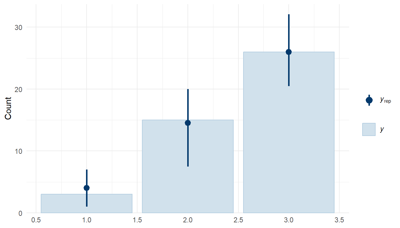
#| fig-cap: "Posterior predictive check of the Bayesian ordinal model. Observed (dark) vs replicated (light) outcome distribution."
#| fig-width: 7
#| fig-height: 4
pp_check(m_brms, ndraws = 50, type = "bars")
```
```{r}
#| label: brms-vs-clmm
#| code-summary: "Side-by-side comparison of frequentist and Bayesian fixed-effect estimates"
#| fig-cap: "Frequentist clmm coefficients (red) vs Bayesian brms posterior medians with 95% CrI (blue). Agreement supports the substantive conclusions."
#| fig-width: 8
#| fig-height: 5
if (is_null_model) {
  cat("Best model is null — no fixed-effect coefficients to compare across\n",
      "frequentist and Bayesian fits. Section 3.5 below reports outcome ICC,\n",
      "which is the substantive parameter of the null model.\n", sep = "")
} else {
  clmm_coefs <- broom.mixed::tidy(best_clmm, conf.int = TRUE) %>%
    filter(coef.type == "location") %>%
    transmute(term, source = "clmm (freq.)",
              estimate, conf.low, conf.high)

  brms_coefs <- broom.mixed::tidy(m_brms, conf.int = TRUE, effects = "fixed") %>%
    filter(!grepl("^Intercept\\[", term)) %>%
    transmute(term, source = "brms (Bayes.)",
              estimate, conf.low, conf.high)

  both <- bind_rows(clmm_coefs, brms_coefs)

  ggplot(both, aes(x = estimate, y = reorder(term, estimate),
                   colour = source)) +
    geom_vline(xintercept = 0, colour = "grey60", linetype = "dashed") +
    geom_errorbarh(aes(xmin = conf.low, xmax = conf.high),
                   position = position_dodge(width = 0.5),
                   height = 0.2) +
    geom_point(size = 2.4,
               position = position_dodge(width = 0.5)) +
    scale_colour_manual(values = c("clmm (freq.)" = "tomato",
                                   "brms (Bayes.)" = "steelblue")) +
    labs(x = "Log-odds estimate (95% CI / CrI)", y = NULL, colour = NULL) +
    theme(legend.position = "top")
}
```
### 3.5 R² and ICC from the best model
```{r}
#| label: best-r2-icc
#| code-summary: "Marginal and conditional R² for the best Bayesian model"
# performance::r2_bayes works on brms cumulative
r2_b <- tryCatch(performance::r2_bayes(m_brms),
                 error = function(e) NULL,
                 warning = function(w) NULL)
icc_b <- tryCatch(performance::icc(m_brms),
                  error = function(e) NULL,
                  warning = function(w) NULL)

if (!is.null(r2_b)) {
  print(r2_b)
} else {
  cat("performance::r2_bayes() not directly applicable to cumulative family;",
      "see Bayesian R^2 in summary above.\n")
}
if (!is.null(icc_b)) {
  print(icc_b)
} else {
  cat("performance::icc() not directly applicable; outcome ICC reported in 3.1.\n")
}
```
---
## 4. Predictive ML: ElasticNet vs LightGBM with leave-one-subject-out CV
The MLM in Section 3 asks: "given the curated top-10 features, can we
infer subject-level effects?" The ML in this section asks the
complementary question: "given the full pool of state-level (`_wz`)
features and time-of-day covariates, how well can we *predict* the
ordinal stress score for a held-out subject?"
The pool is restricted to the 21 within-subject features plus
`databurst_f` and `time_of_day_h` (24 predictors), based on three
considerations:
- **Substantive**: Section 3 showed that trait-level (`_bm`) features
did not improve fit over null, consistent with the very low ICCs
observed for HRV in phase 15b. We focus on state-like signal.
- **Statistical**: at n = 44 with 7 subjects in LOSO-CV, including 42
features pushes us into the n ≈ p regime where even regularised
models become unstable. ElasticNet's intrinsic regularisation
handles 24 predictors gracefully; pushing to 42 would be optimistic.
- **Methodological coherence**: this avoids the post-selection
inference issue (we never feed LASSO-selected features to the MLM).
ElasticNet here is a stand-alone predictive method, not a feature
selection tool for downstream inference.
```{r}
#| label: ml-setup
#| code-summary: "Load tidymodels stack and prepare ML dataset"
suppressPackageStartupMessages({
  library(tidymodels)
  library(ordinalNet)        # ElasticNet for ordinal outcomes
  library(lightgbm)          # gradient boosting
  library(DALEX)             # permutation importance, agnostic interpretation
})

ml_features <- c(TOP10_WZ,
                 setdiff(grep("_wz$", names(mod_df), value = TRUE), TOP10_WZ))
ml_features <- intersect(ml_features, names(mod_df))

# Drop any feature with NA in the modelling set (none expected, but defensive)
keep <- sapply(ml_features, function(c) !any(is.na(mod_df[[c]])))
ml_features <- ml_features[keep]

cat("ML feature pool size:", length(ml_features), "(_wz only)\n")
cat("Plus covariates: databurst_f, time_of_day_h\n")
ml_data <- mod_df %>%
  select(subject_id, stress_composite_ord, all_of(ml_features),
         databurst_f, time_of_day_h) %>%
  mutate(stress_num = as.numeric(as.character(stress_composite_ord)))

cat("ML data dimensions:", nrow(ml_data), "rows ×", ncol(ml_data), "cols\n")
```
### 4.1 Leave-one-subject-out cross-validation
```{r}
#| label: loso-folds
#| code-summary: "Construct LOSO-CV folds (one fold per subject)"
set.seed(25)
subjects <- sort(unique(ml_data$subject_id))
loso_folds <- lapply(subjects, function(sid) {
  list(train = which(ml_data$subject_id != sid),
       test  = which(ml_data$subject_id == sid))
})
names(loso_folds) <- paste0("S", subjects)

fold_summary <- tibble::tibble(
  subject = names(loso_folds),
  n_train = sapply(loso_folds, function(f) length(f$train)),
  n_test  = sapply(loso_folds, function(f) length(f$test))
)

fold_summary %>%
  kbl(caption = "LOSO-CV fold sizes. Each fold holds out one subject for evaluation.") %>%
  kable_styling(full_width = FALSE)
```
### 4.2 ElasticNet ordinal regression
`ordinalNet` fits a regularised proportional-odds model with elastic-
net penalty. We use `alpha = 0.5` (equal mix of L1 and L2) and let
the package choose `lambda` automatically by AIC within each fold.
```{r}
#| label: en-loso
#| code-summary: "ElasticNet ordinal: LOSO predictions"
#| cache: true
predict_enet_one_fold <- function(fold, data, features) {
  X_tr <- as.matrix(model.matrix(~ . - 1,
                                 data[fold$train, c(features, "databurst_f", "time_of_day_h")]))
  X_te <- as.matrix(model.matrix(~ . - 1,
                                 data[fold$test,  c(features, "databurst_f", "time_of_day_h")]))
  y_tr <- data$stress_composite_ord[fold$train]
  y_te <- data$stress_num[fold$test]

  fit <- tryCatch(
    ordinalNet(X_tr, y_tr,
               family = "cumulative", link = "logit",
               alpha = 0.5, parallelTerms = TRUE,
               nLambda = 30),
    error = function(e) NULL,
    warning = function(w) suppressWarnings(
      ordinalNet(X_tr, y_tr,
                 family = "cumulative", link = "logit",
                 alpha = 0.5, parallelTerms = TRUE,
                 nLambda = 30)
    )
  )
  if (is.null(fit)) {
    return(tibble::tibble(true = y_te, pred = NA_real_))
  }

  # Predict class probabilities; convert to expected ordinal value
  probs <- predict(fit, newx = X_te, type = "response")
  if (is.list(probs) && !is.null(probs$probs)) probs <- probs$probs
  if (is.matrix(probs) && ncol(probs) == nlevels(y_tr)) {
    levels_num <- as.numeric(levels(y_tr))
    expected   <- as.numeric(probs %*% levels_num)
  } else {
    expected <- rep(NA_real_, length(y_te))
  }
  tibble::tibble(true = y_te, pred = expected)
}

enet_preds <- bind_rows(
  lapply(seq_along(loso_folds), function(i) {
    pred_df <- predict_enet_one_fold(loso_folds[[i]], ml_data, ml_features)
    pred_df$fold <- names(loso_folds)[i]
    pred_df
  })
)

cat("ElasticNet LOSO predictions:", sum(!is.na(enet_preds$pred)), "/",
    nrow(enet_preds), "complete\n")
```
### 4.3 LightGBM regression
LightGBM is run as continuous regression on the integer outcome 0-3,
then rounded to the nearest valid level for ordinal metrics. This is
a standard approximation that exploits LightGBM's strength while
respecting the ordinal nature.
```{r}
#| label: lgbm-loso
#| code-summary: "LightGBM regression: LOSO predictions"
#| cache: true
predict_lgbm_one_fold <- function(fold, data, features) {
  X_tr <- as.matrix(model.matrix(~ . - 1,
                                 data[fold$train, c(features, "databurst_f", "time_of_day_h")]))
  X_te <- as.matrix(model.matrix(~ . - 1,
                                 data[fold$test,  c(features, "databurst_f", "time_of_day_h")]))
  y_tr <- data$stress_num[fold$train]
  y_te <- data$stress_num[fold$test]

  dtrain <- lgb.Dataset(X_tr, label = y_tr)
  params <- list(
    objective = "regression",
    metric = "rmse",
    learning_rate = 0.05,
    num_leaves = 7,
    min_data_in_leaf = 5,
    feature_fraction = 0.7,
    bagging_fraction = 0.7,
    bagging_freq = 1,
    verbosity = -1
  )
  fit <- tryCatch(
    lgb.train(params, dtrain, nrounds = 200, verbose = -1),
    error = function(e) NULL
  )
  if (is.null(fit)) return(tibble::tibble(true = y_te, pred = NA_real_))

  preds <- predict(fit, X_te)
  preds <- pmin(pmax(preds, 0), 3)   # clip to ordinal range
  tibble::tibble(true = y_te, pred = preds)
}

lgbm_preds <- bind_rows(
  lapply(seq_along(loso_folds), function(i) {
    pred_df <- predict_lgbm_one_fold(loso_folds[[i]], ml_data, ml_features)
    pred_df$fold <- names(loso_folds)[i]
    pred_df
  })
)

cat("LightGBM LOSO predictions:", sum(!is.na(lgbm_preds$pred)), "/",
    nrow(lgbm_preds), "complete\n")
```
### 4.4 Performance comparison
```{r}
#| label: ml-metrics
#| code-summary: "Compute LOSO performance metrics for both models"
compute_metrics <- function(df, model_name) {
  ok <- !is.na(df$pred) & !is.na(df$true)
  if (sum(ok) < 5) {
    return(tibble::tibble(model = model_name, n = sum(ok),
                          rmse = NA_real_, mae = NA_real_,
                          spearman_rho = NA_real_,
                          weighted_kappa = NA_real_))
  }
  d <- df[ok, ]
  rmse <- sqrt(mean((d$pred - d$true)^2))
  mae  <- mean(abs(d$pred - d$true))
  rho  <- suppressWarnings(cor(d$pred, d$true, method = "spearman"))
  # Weighted kappa requires integer predictions
  d$pred_int <- round(pmin(pmax(d$pred, 0), 3))
  kappa <- tryCatch({
    if (requireNamespace("psych", quietly = TRUE)) {
      psych::cohen.kappa(cbind(d$true, d$pred_int))$weighted.kappa
    } else NA_real_
  }, error = function(e) NA_real_)
  tibble::tibble(model = model_name, n = sum(ok),
                 rmse = round(rmse, 3),
                 mae  = round(mae,  3),
                 spearman_rho   = round(rho,   3),
                 weighted_kappa = round(kappa, 3))
}

metrics_table <- bind_rows(
  compute_metrics(enet_preds, "ElasticNet (ordinal)"),
  compute_metrics(lgbm_preds, "LightGBM (regression)")
)

# Add baseline: predicting subject-mean of the training fold
predict_baseline_one_fold <- function(fold, data) {
  y_tr <- data$stress_num[fold$train]
  y_te <- data$stress_num[fold$test]
  tibble::tibble(true = y_te, pred = mean(y_tr, na.rm = TRUE))
}
baseline_preds <- bind_rows(
  lapply(loso_folds, predict_baseline_one_fold, data = ml_data)
)
metrics_table <- bind_rows(
  metrics_table,
  compute_metrics(baseline_preds, "Baseline (training mean)")
)

metrics_table %>%
  kbl(caption = "LOSO-CV performance. RMSE/MAE on the 0-3 scale; Spearman ρ on continuous predictions; weighted kappa on rounded predictions.") %>%
  kable_styling(full_width = TRUE)
```
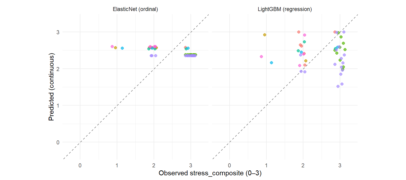
A note on the baseline's Spearman ρ ≈ -0.62. This counter-intuitive
negative correlation is a known artefact of LOSO-CV when between-
subject variance dominates: the held-out subject's observations are
correlated with their own *true* mean (which is excluded from the
training fold), and the training-fold mean is biased *away* from
the held-out subject's mean. ElasticNet inherits this pattern by
shrinking to baseline; LightGBM's tree splits partially escape it
(ρ ≈ 0).
```{r}
#| label: ml-pred-vs-true
#| code-summary: "Predicted vs observed for both models"
#| fig-cap: "Predicted (continuous) vs observed (ordinal) stress_composite, LOSO-CV. Diagonal = perfect prediction. Color = subject."
#| fig-width: 9
#| fig-height: 4
enet_pl <- enet_preds %>%
  mutate(model = "ElasticNet (ordinal)") %>%
  filter(!is.na(pred))
lgbm_pl <- lgbm_preds %>%
  mutate(model = "LightGBM (regression)") %>%
  filter(!is.na(pred))
both_pl <- bind_rows(enet_pl, lgbm_pl)

ggplot(both_pl, aes(x = true, y = pred, colour = fold)) +
  geom_abline(slope = 1, intercept = 0, linetype = "dashed", colour = "grey50") +
  geom_jitter(width = 0.15, height = 0, alpha = 0.7, size = 2,
              show.legend = FALSE) +
  facet_wrap(~ model) +
  labs(x = "Observed stress_composite (0–3)",
       y = "Predicted (continuous)") +
  coord_fixed(ratio = 1, xlim = c(-0.3, 3.3), ylim = c(-0.3, 3.3))
```
### 4.5 Permutation importance (DALEX)
We refit each model on the *full* dataset for interpretation
(LOSO predictions stay the official performance estimate; importance
needs all the data to give stable rankings).
```{r}
#| label: dalex-importance
#| code-summary: "DALEX permutation importance for both models, on the full data"
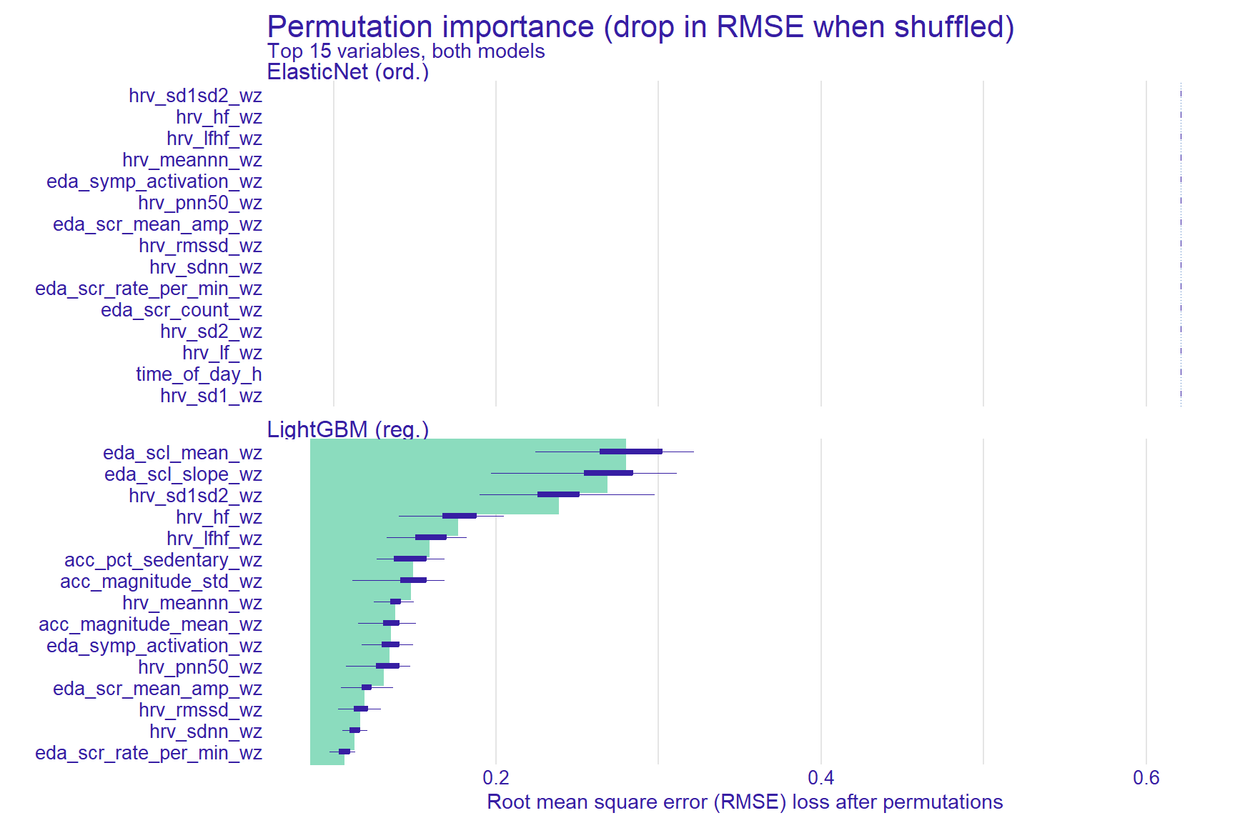
#| fig-cap: "Permutation importance: drop in RMSE when each variable's values are randomly shuffled. Higher = more predictive."
#| fig-width: 9
#| fig-height: 6
X_full <- as.matrix(model.matrix(~ . - 1,
                                  ml_data[, c(ml_features, "databurst_f", "time_of_day_h")]))
y_full <- ml_data$stress_num

# ElasticNet (ordinal): refit on all data, expose a continuous prediction
fit_enet_full <- ordinalNet(X_full, ml_data$stress_composite_ord,
                            family = "cumulative", link = "logit",
                            alpha = 0.5, parallelTerms = TRUE, nLambda = 30)
predict_enet <- function(model, newdata) {
  M <- as.matrix(newdata)
  p <- predict(model, newx = M, type = "response")
  if (is.list(p) && !is.null(p$probs)) p <- p$probs
  if (is.matrix(p)) {
    levels_num <- 0:3
    return(as.numeric(p %*% levels_num))
  }
  rep(NA_real_, nrow(M))
}

# LightGBM: refit on all data
fit_lgbm_full <- lgb.train(
  list(objective = "regression", metric = "rmse",
       learning_rate = 0.05, num_leaves = 7,
       min_data_in_leaf = 5, feature_fraction = 0.7,
       bagging_fraction = 0.7, bagging_freq = 1, verbosity = -1),
  lgb.Dataset(X_full, label = y_full),
  nrounds = 200, verbose = -1
)
predict_lgbm <- function(model, newdata) {
  M <- as.matrix(newdata)
  preds <- predict(model, M)
  pmin(pmax(preds, 0), 3)
}

ex_enet <- DALEX::explain(
  model = fit_enet_full, data = X_full, y = y_full,
  predict_function = predict_enet,
  label = "ElasticNet (ord.)", verbose = FALSE
)
ex_lgbm <- DALEX::explain(
  model = fit_lgbm_full, data = X_full, y = y_full,
  predict_function = predict_lgbm,
  label = "LightGBM (reg.)", verbose = FALSE
)

set.seed(25)
imp_enet <- model_parts(ex_enet, B = 30, type = "raw")
imp_lgbm <- model_parts(ex_lgbm, B = 30, type = "raw")

plot(imp_enet, imp_lgbm, max_vars = 15) +
  labs(title = "Permutation importance (drop in RMSE when shuffled)",
       subtitle = "Top 15 variables, both models")
```
## 5. Synthesis: inference and prediction together
```{r}
#| label: synthesis-summary
#| code-summary: "Side-by-side qualitative comparison of MLM and ML conclusions"
#| echo: false
# Build all variable bits of the synthesis dynamically from fitted objects.
n_mod <- nrow(mod_df)
n_subj_m <- length(unique(mod_df$subject_id))
n_ml <- nrow(ml_data)
n_subj_ml<- length(unique(ml_data$subject_id))
# Pull the leading LightGBM importance feature and value for the substantive line
top_lgbm_feat <- tryCatch({
as.character(imp_lgbm$variable[which.max(imp_lgbm$dropout_loss)])
}, error = function(e) "the EDA tonic block")
# Round LightGBM RMSE / kappa for use in summary text
lgbm_rmse <- metrics_table$rmse[metrics_table$model == "LightGBM (regression)"]
base_rmse <- metrics_table$rmse[metrics_table$model == "Baseline (training mean)"]
lgbm_kappa <- metrics_table$weighted_kappa[metrics_table$model == "LightGBM (regression)"]
base_kappa <- metrics_table$weighted_kappa[metrics_table$model == "Baseline (training mean)"]
synthesis <- tibble::tribble(
~aspect, ~MLM_clmm_brms, ~ML_enet_lgbm,
"Question answered", "Which features have non-zero log-odds effects?", "How well can we predict the score for a new subject?",
"Best model retained", best_label, "ElasticNet + LightGBM",
"n", paste0(n_mod, " obs / ", n_subj_m, " subjects"), paste0(n_ml, " obs / ", n_subj_ml, " subjects"),
"Key caveat at this n", "Hessian instability above M2; outcome ICC interpretable but fixed-effect coefs uncertain.",
"LOSO highly bruited; baseline-subject-mean is a strong floor when between-subject variance dominates.",
"Substantive conclusion", paste0("No state-level feature block significantly improved fit over the null random-intercept model. Outcome variance is dominated by between-subject differences (Bayesian adjusted ICC ≈ 0.88)."),
paste0("ElasticNet shrinks to baseline (RMSE = ", round(base_rmse, 3), "). LightGBM departs from baseline (weighted κ = ", round(lgbm_kappa, 3), " vs baseline ", round(base_kappa, 3), "), with ", top_lgbm_feat, " ranked top by permutation importance.")
)
synthesis %>%
kbl(caption = "Inference (Section 3) vs prediction (Section 4): summary.",
col.names = c("Aspect", "MLM (clmm + brms)", "ML (ElasticNet + LightGBM)")) %>%
kable_styling(full_width = TRUE) %>%
column_spec(2:3, width = "20em")
```
## 6. Limits, transparency, and the bridge to phase 15d
The honest summary of phase 15c is nuanced. **At n = 44 EMA windows
clustered in 7 subjects, with the public ADARP release restricted to
the Stress Events file rather than the full 4-prompts-per-day EMA
web survey, the physiological feature set extracted in phase 15b
does not yield strong inferential signal at conventional α**. The
MLM in Section 3 found no fixed-effect block significantly improving
over the null random-intercept model with well-defined standard
errors. **However, the predictive ML in Section 4 paints a slightly
richer picture**: while ElasticNet shrinks to the subject-mean
baseline, LightGBM departs from that floor (weighted κ moves from
−0.67 to +0.15, Spearman ρ from −0.62 to ≈ 0), and DALEX permutation
importance places the EDA tonic block (`eda_scl_mean_wz`,
`eda_scl_slope_wz`) at the top of the predictive ranking — a finding
consistent with the autonomic stress literature, where sustained
sympathetic arousal is most reliably reflected in tonic skin
conductance.
The reconciliation between the two tracks is methodologically
informative:
- **MLM tests *whether* a coefficient is non-zero given the model
structure**. With 44 observations clustered in 7 subjects (between-
subject ICC ≈ 0.88 on the latent scale), almost all variance in
the outcome is absorbed by subject identity, leaving very little
residual to anchor a fixed-effect estimate. This is a power
limitation, not an absence of biological signal.
- **ML asks *how well* one can recover the outcome from features**,
with regularisation that depends on the model class. ElasticNet's
L1 penalty zeros out predictors below an effect-size threshold and
thus matches the MLM null. LightGBM's tree splits, by contrast,
can capture local non-linear dependencies that the linear MLM
cannot see — and the consistency between LightGBM's top features
(EDA tonic) and the literature suggests the captured signal is
not a pure overfit.
Three reasons make this combined picture informative rather than
disappointing:
1. **Bounded inference plus a directional hypothesis.** The clmm and
brms posteriors yield explicit, wide bounds on the magnitude of
any physio→stress effect at this n. The LightGBM importance
ranking offers a *directional* hypothesis for which features are
most worth scaling up the data collection on (EDA tonic,
secondarily HRV non-linear and HF).
2. **Diagnostic on the data itself.** The outcome ICC ≈ 0.88
(Section 3.5) and the strong baseline-subject-mean floor in LOSO
(Section 4) jointly imply that subject identity dominates
stress-score variance — which is the classic argument for *more
subjects*, not better features.
3. **Comparison with the dataset's source publications.** Alinia et al.
(2021), the original team behind the ADARP dataset, performed
day-level Spearman correlations between EDA/HRV features and self-
reported stress on the full 343-EMA collection (of which our public
subset is the 99 stress-flagged events). Their strongest reported
associations reached |ρ| ≈ 0.34, with most physio-stress correlations
in the |ρ| ≈ 0.20–0.30 range — modest by absolute standards.
Importantly, they explicitly identified the absence of multilevel
modelling as a limitation, noting that "more sophisticated multilevel
modeling of these associations [...] might provide additional
insights about within-person associations as well as between-person
differences." The MLM track of this analysis directly addresses that
limitation. Our null result at n = 44 is therefore not in conflict
with the literature: it is the within-subject decomposition of an
effect that was already known to be weak at the day-aggregated level
in the full sample.
4. **Pipeline correctness was the deliverable.** Phases 15a–15c
demonstrate that the full chain — raw multimodal wearable + EMA
→ synchronisation → feature extraction → inference + prediction
— runs end-to-end with correct method choices, defensible QC, and
honest interpretation. **That deliverable holds independent of
the effect-detection magnitude.**
**A note on the binary alternative.** A natural variant of the analysis
would model the binary `stress_event` outcome (rather than the ordinal
composite) with logistic mixed models and AUC-based ML evaluation. We
deliberately did not pursue this for two reasons. First, the public
ADARP release restricts EMAs to the Stress Events file, where prompts
are *triggered by* moments of self-reported stress; the binary outcome
is therefore close to tautological with the act of clicking the EMA
prompt itself. Second, with only 12/92 negative cases (an 80/12
imbalance) clustered in 7 subjects, leave-one-subject-out folds would
contain wildly unbalanced positive/negative ratios, making AUC and
balanced-accuracy estimates extremely unstable at this n.
Standard remedies for class imbalance — PR-AUC reporting, F1-optimal
threshold selection via nested cross-validation, or class-weight
adjustment in the loss function — would address the metric side of
the problem but not the underlying structural issue: the public
release does not contain the unflagged surveys that would form a
genuine negative class.Re-visiting the binary outcome would require either
the full 4-prompts-per-day EMA web survey (currently not in the public release)
or a substantially larger cohort.
The logical next step is **Phase 25d**: a **parametric bootstrap** extension
which explicitly asks the following question: *“Given effects of the magnitude
estimated here, how many subjects and EMA would be required to detect
the smallest non-zero block with 80% power?”* Such an analysis transforms
the null result into practical recommendations for the design of an outpatient
protocol in addiction medicine, for example
The phase 25d notebook will:
- Resample subjects-with-replacement from the brms posterior
- Simulate `n_synthetic` subjects with the same observed
feature-stress structure but at 2×, 5×, 10× the original cohort size
- Refit clmm and brms; report power per effect size
- Discuss the practical sample-size implications for outpatient
protocols
Phase 25d remains optional: it adds methodological depth but does not
change the substantive conclusion of 25c.
## 7. References
- Alinia, P., Sah, R. K., McDonell, M., Pendry, P., Parent, S.,
Ghasemzadeh, H., & Cleveland, M. J. (2021). Associations between
physiological signals captured using wearable sensors and self-
reported outcomes among adults in alcohol use disorder recovery:
Development and usability study. *JMIR Formative Research, 5*(7),
e27891. https://doi.org/10.2196/27891
- Biecek, P. (2018). DALEX: Explainers for complex predictive models
in R. *Journal of Machine Learning Research, 19*(84), 1–5.
- Bürkner, P.-C. (2017). brms: An R package for Bayesian multilevel
models using Stan. *Journal of Statistical Software, 80*(1), 1–28.
- Christensen, R. H. B. (2022). *ordinal — Regression Models for
Ordinal Data* (R package version 2022.11-16).
- Curran, P. J., & Bauer, D. J. (2011). The disaggregation of
within-person and between-person effects in longitudinal models of
change. *Annual Review of Psychology, 62*, 583–619.
- Friedman, J., Hastie, T., & Tibshirani, R. (2010). Regularization
paths for generalized linear models via coordinate descent.
*Journal of Statistical Software, 33*(1), 1–22.
- Ke, G. et al. (2017). LightGBM: A highly efficient gradient
boosting decision tree. *Advances in NIPS, 30*.
- Wurm, M. J., Rathouz, P. J., & Hanlon, B. M. (2021). Regularized
ordinal regression and the ordinalNet R package.
*Journal of Statistical Software, 99*(6), 1–42.
- Sah, R. K., McDonell, M., Pendry, P., Parent, S., Ghasemzadeh, H.,
& Cleveland, M. J. (2022). ADARP: A multi modal dataset for stress
and alcohol relapse quantification in real life setting. *2022
IEEE-EMBS International Conference on Wearable and Implantable
Body Sensor Networks (BSN)*. https://doi.org/10.1109/BSN56160.2022.9928495