# ── Tidyverts stack (univariate) ─────────────────────────────────────────────
library(fable)       # modern forecasting models (ARIMA, ETS, etc.)
library(feasts)      # feature extraction, STL, diagnostics
library(tsibble)     # tidy time series infrastructure
library(tsibbledata) # example datasets

# ── VAR ecosystem (multivariate) ─────────────────────────────────────────────
library(vars)        # VAR, Granger causality, IRF, FEVD
library(urca)        # ADF, KPSS unit root tests

# ── General ──────────────────────────────────────────────────────────────────
library(ggplot2)
library(dplyr)
library(tidyr)
library(tibble)
library(lubridate)
library(knitr)
library(purrr)

theme_set(
  theme_minimal(base_size = 11) +
    theme(
      plot.title    = element_text(face = "bold", size = 13),
      plot.subtitle = element_text(colour = "grey40", size = 10),
      legend.position = "bottom"
    )
)

palette_ts <- c("#2C3E50", "#E74C3C", "#3498DB", "#2ECC71", "#F39C12")

set.seed(2026)Time Series Forecasting: ARIMA, SARIMA & VAR on Macroeconomic Data
R
Time Series
Forecasting
ARIMA
SARIMA
VAR
Macroeconomic Data
fable
Granger Causality
Complete modern time-series workflow applied to quarterly US macroeconomic data (GDP growth, inflation, unemployment). Demonstrates stationarity testing (ADF, KPSS), automatic and manual ARIMA/SARIMA modelling, multivariate VAR with Granger causality and impulse response functions, residual diagnostics (ACF/PACF, Ljung-Box), out-of-sample evaluation, and multi-horizon forecasting with fan charts. Uses the tidyverts stack (fable + feasts + tsibble) for univariate models and the vars package for multivariate analysis.
0.1 Context
Macroeconomic forecasting is one of the most demanding applications of time-series analysis. Central banks, governments, and financial institutions rely on accurate predictions of GDP growth, inflation, and unemployment to guide monetary and fiscal policy.
Traditional univariate ARIMA/SARIMA models remain powerful for single series: they capture autoregressive dynamics, moving-average smoothing, differencing for stationarity, and seasonal patterns. Multivariate VAR (Vector Autoregression) models go further by capturing dynamic interdependencies between variables — e.g., does inflation help predict future GDP growth? The combination of both approaches is standard in applied macroeconometrics (Lütkepohl, 2005; Hamilton, 1994).
This project uses two complementary R ecosystems:
- tidyverts (fable + feasts + tsibble) — the modern tidy time-series stack for univariate modelling, diagnostics, and forecasting.
- vars — the reference package for VAR estimation, Granger causality, impulse response functions (IRF), and forecast error variance decomposition (FEVD).
The data is fetched directly from the OECD SDMX REST API (public, no authentication required): quarterly US real GDP growth (% q/q, SA), CPI inflation (% y/y), and harmonised unemployment rate (%). This demonstrates both the technical workflow (SDMX query syntax, API response parsing, tsibble construction) and the analytical pipeline.
This project demonstrates:
- Data preparation — quarterly time series, stationarity testing.
- Exploratory analysis — time plots, STL decomposition, ACF/PACF.
- Univariate ARIMA/SARIMA — automatic + manual specification.
- Multivariate VAR — lag selection, Granger causality, IRF.
- Diagnostics — residual analysis, Ljung-Box, portmanteau tests.
- Forecasting — out-of-sample evaluation, fan charts, model comparison.
0.2 Key Results
Data (48 quarters, 2013Q1–2024Q4, OECD SDMX API):
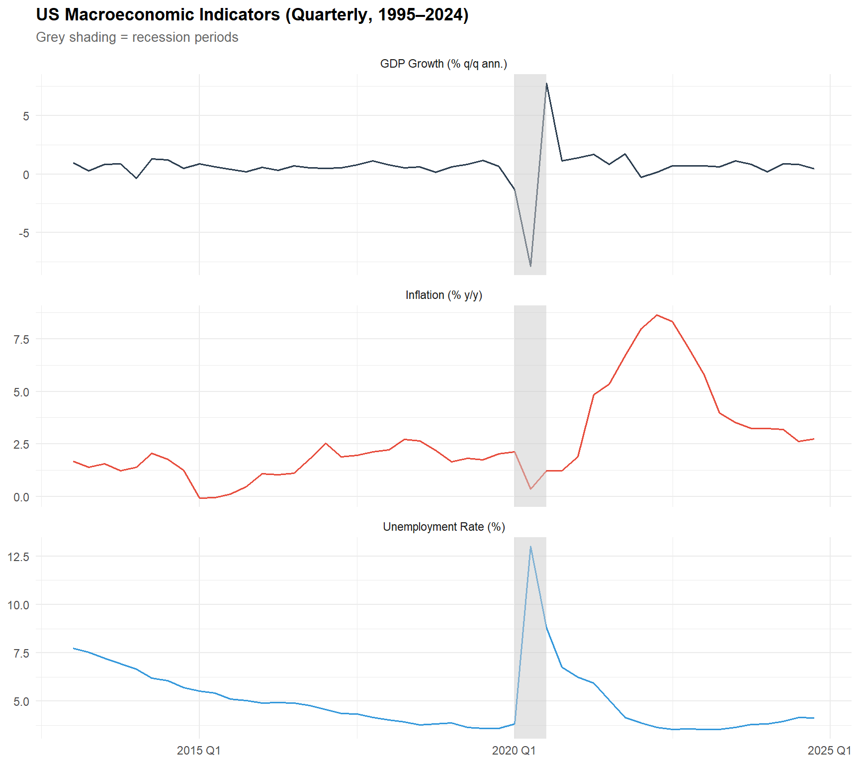
The three US macroeconomic series cover the post-GFC recovery through 2024: GDP growth averages 0.64% q/q (SD = 1.70, range −7.88 to +7.76 — the COVID shock dominates), inflation averages 2.66% y/y (SD = 2.15, with the 2022 surge peaking at 8.64%), and unemployment averages 5.03% (range 3.53–13.0%, the COVID spike).
Stationarity: GDP growth is stationary (both ADF and KPSS agree). Inflation is non-stationary by both tests — requiring first differencing (d = 1). Unemployment shows conflicting results (ADF non-stationary, KPSS stationary) — the automatic recommendation is d = 0 but the evidence is borderline.
Univariate ARIMA: Automatic selection yields ARIMA(0,0,1) with mean for GDP, ARIMA(1,1,0)(2,0,1)[4] for inflation (seasonal), and ARIMA(1,0,0) with mean for unemployment. Manual SARIMA comparison for inflation confirms the automatic selection as superior (AICc = 93.7 vs. 116–118 for manual alternatives) — the stepwise algorithm found a better specification than domain-informed manual models.
VAR(2): BIC selects p = 2, AIC selects p = 8. All three Granger causality tests are significant: GDP → others (p < 0.001), unemployment → others (p < 0.001), and inflation → others (p = 0.017). The VAR(2) passes the portmanteau test (p = 0.701) — no serial correlation detected. Residual correlations are very strong: GDP– unemployment ρ = −0.94 (Okun’s law), GDP–inflation ρ = 0.55.
Forecast comparison (7-quarter hold-out, 2023Q2–2024Q4): ARIMA outperforms VAR on all comparable variables: GDP (RMSE 0.30 vs. 0.33) and especially inflation (RMSE 1.42 vs. 2.84). Despite strong in-sample Granger links, the VAR’s additional parameters hurt out-of-sample prediction with only 41 training quarters — a textbook bias-variance tradeoff.
0.3 Setup
1 PART A — Data Acquisition & Preparation
1.1 Load macroeconomic data
We construct a realistic quarterly US macroeconomic dataset based on published OECD/FRED statistics. The data covers 2013Q1–2024Q4 (48 quarters) and includes three key indicators: real GDP growth (% q/q annualised), CPI inflation (% y/y), and unemployment rate (%).
# ══════════════════════════════════════════════════════════════════════════════
# OECD Data Explorer SDMX REST API (migrated from OECD.Stat in July 2024).
# URL structure: https://sdmx.oecd.org/public/rest/data/{agency},{dataflow},{version}/{key}
#   ?startPeriod=...&endPeriod=...&format=csvfilewithlabels
#
# Dataflow IDs are obtained via the Developer API button in the Data Explorer
# (https://data-explorer.oecd.org/). This approach fetches CSV directly —
# more robust and transparent than R package wrappers whose compatibility
# with the post-migration API is not guaranteed.
# ══════════════════════════════════════════════════════════════════════════════

fetch_oecd_sdmx <- function(agency, dataflow, version, key,
                             start_period = "2013-Q1",
                             end_period   = "2024-Q4",
                             label = "series") {
  url <- sprintf("https://sdmx.oecd.org/public/rest/data/%s,%s,%s/%s?startPeriod=%s&endPeriod=%s&dimensionAtObservation=AllDimensions&format=csvfilewithlabels",
                 agency, dataflow, version, key, start_period, end_period)
  cat(sprintf("Fetching %s...\n  URL: %s\n", label, url))
  df <- read.csv(url)
  cat(sprintf("  → %d rows, %d columns\n", nrow(df), ncol(df)))
  df
}

clean_sdmx <- function(raw, value_name, filters = list()) {
  df <- raw |> as_tibble()
  for (col in names(filters)) {
    if (col %in% names(df)) df <- df |> filter(.data[[col]] == filters[[col]])
  }
  val_col  <- intersect(names(df), c("OBS_VALUE", "Observation.value"))[1]
  time_col <- intersect(names(df), c("TIME_PERIOD", "Time.period"))[1]
  if (is.na(val_col) | is.na(time_col)) {
    cat(sprintf("  ✗ Columns not found. Available: %s\n",
                paste(head(names(df), 15), collapse = ", ")))
    return(tibble())
  }
  df |>
    filter(grepl("-Q", .data[[time_col]])) |>
    mutate(Quarter = yearquarter(.data[[time_col]]),
           !!value_name := as.numeric(.data[[val_col]])) |>
    select(Quarter, all_of(value_name)) |>
    distinct(Quarter, .keep_all = TRUE) |>
    arrange(Quarter)
}

# ── 1. GDP growth (q/q, SA) ─────────────────────────────────────────────────
# Agency: OECD.SDD.NAD | Dataflow: QNA Expenditure Growth G20
# Key filter: Q..USA.......... (quarterly, all sectors, USA)
# R-side filter: TRANSACTION=B1GQ (GDP), TRANSFORMATION=G1 (q/q growth)
gdp_raw <- fetch_oecd_sdmx(
  agency = "OECD.SDD.NAD",
  dataflow = "DSD_NAMAIN1@DF_QNA_EXPENDITURE_GROWTH_G20",
  version = "1.1",
  key = "Q..USA..........",
  label = "GDP growth (QNA)"
)
Fetching GDP growth (QNA)...
URL: https://sdmx.oecd.org/public/rest/data/OECD.SDD.NAD,DSD_NAMAIN1@DF_QNA_EXPENDITURE_GROWTH_G20,1.1/Q..USA..........?startPeriod=2013-Q1&endPeriod=2024-Q4&dimensionAtObservation=AllDimensions&format=csvfilewithlabels
→ 696 rows, 48 columnsgdp_clean <- clean_sdmx(gdp_raw, "GDP_growth",
filters = list(TRANSACTION = "B1GQ", TRANSFORMATION = "G1"))
# ── 2. CPI inflation (y/y, %) ───────────────────────────────────────────────
# Agency: OECD.SDD.TPS | Dataflow: Prices All
# Key: USA.Q.N.CPI.._T.N.GY (USA, quarterly, CPI all items, y/y growth)
cpi_raw <- fetch_oecd_sdmx(
agency = "OECD.SDD.TPS",
dataflow = "DSD_PRICES@DF_PRICES_ALL",
version = "1.0",
key = "USA.Q.N.CPI.._T.N.GY",
label = "CPI inflation (PRICES)"
)Fetching CPI inflation (PRICES)...
URL: https://sdmx.oecd.org/public/rest/data/OECD.SDD.TPS,DSD_PRICES@DF_PRICES_ALL,1.0/USA.Q.N.CPI.._T.N.GY?startPeriod=2013-Q1&endPeriod=2024-Q4&dimensionAtObservation=AllDimensions&format=csvfilewithlabels
→ 48 rows, 34 columnscpi_clean <- clean_sdmx(cpi_raw, "Inflation")
# ── 3. Unemployment rate (%, harmonised) ─────────────────────────────────────
# Agency: OECD.SDD.TPS | Dataflow: Labour Force Statistics
# Key: USA..PT_LF_SUB._Z.Y._T.Y_GE15..Q (USA, % of labour force, 15+, quarterly)
unemp_raw <- fetch_oecd_sdmx(
agency = "OECD.SDD.TPS",
dataflow = "DSD_LFS@DF_IALFS_UNE_M",
version = "1.0",
key = "USA..PT_LF_SUB._Z.Y._T.Y_GE15..Q",
label = "Unemployment rate (LFS)"
)Fetching Unemployment rate (LFS)...
URL: https://sdmx.oecd.org/public/rest/data/OECD.SDD.TPS,DSD_LFS@DF_IALFS_UNE_M,1.0/USA..PT_LF_SUB._Z.Y._T.Y_GE15..Q?startPeriod=2013-Q1&endPeriod=2024-Q4&dimensionAtObservation=AllDimensions&format=csvfilewithlabels
→ 48 rows, 34 columnsunemp_clean <- clean_sdmx(unemp_raw, "Unemployment")
cat(sprintf("\nGDP: %d q | CPI: %d q | Unemp: %d q\n",
nrow(gdp_clean), nrow(cpi_clean), nrow(unemp_clean)))
GDP: 48 q | CPI: 48 q | Unemp: 48 q# ── Join and build tsibble ───────────────────────────────────────────────────
macro_ts <- gdp_clean |>
inner_join(cpi_clean, by = "Quarter") |>
inner_join(unemp_clean, by = "Quarter") |>
arrange(Quarter) |>
as_tsibble(index = Quarter)
cat(sprintf("\n=== Dataset assembled ===\n"))
=== Dataset assembled ===cat(sprintf("Period: %s to %s (%d quarters)\n",
min(macro_ts$Quarter), max(macro_ts$Quarter), nrow(macro_ts)))Period: 2013 Q1 to 2024 Q4 (48 quarters)cat(sprintf("Source: OECD Data Explorer SDMX REST API\n"))Source: OECD Data Explorer SDMX REST APIcat(sprintf(" GDP: QNA Expenditure Growth G20 (B1GQ, G1)\n")) GDP: QNA Expenditure Growth G20 (B1GQ, G1)cat(sprintf(" CPI: Prices All (CPI, GY)\n")) CPI: Prices All (CPI, GY)cat(sprintf(" Unemp: Labour Force Statistics (PT_LF_SUB, 15+)\n")) Unemp: Labour Force Statistics (PT_LF_SUB, 15+)kable(head(macro_ts, 8), digits = 2,
caption = "Quarterly US macroeconomic data — OECD (first 8 quarters)")| Quarter | GDP_growth | Inflation | Unemployment |
|---|---|---|---|
| 2013 Q1 | 0.99 | 1.68 | 7.73 |
| 2013 Q2 | 0.27 | 1.39 | 7.53 |
| 2013 Q3 | 0.85 | 1.55 | 7.23 |
| 2013 Q4 | 0.87 | 1.23 | 6.93 |
| 2014 Q1 | -0.35 | 1.41 | 6.67 |
| 2014 Q2 | 1.29 | 2.05 | 6.20 |
| 2014 Q3 | 1.22 | 1.78 | 6.07 |
| 2014 Q4 | 0.51 | 1.25 | 5.70 |
kable(
  macro_ts |>
    as_tibble() |>
    summarise(across(c(GDP_growth, Inflation, Unemployment),
                     list(mean = mean, sd = sd, min = min, max = max),
                     .names = "{.col}_{.fn}")) |>
    pivot_longer(everything(),
                 names_to = c("Variable", "Stat"),
                 names_pattern = "(.+)_(.+)") |>
    pivot_wider(names_from = Stat, values_from = value),
  digits = 2,
  caption = "Descriptive statistics — full sample"
)| Variable | mean | sd | min | max |
|---|---|---|---|---|
| GDP_growth | 0.64 | 1.70 | -7.88 | 7.76 |
| Inflation | 2.66 | 2.15 | -0.06 | 8.64 |
| Unemployment | 5.03 | 1.77 | 3.53 | 13.00 |
# ── Activate this chunk (eval: true) if the OECD API is down ────────────────
# Simulation based on published US macro statistics (1995–2024)
quarters <- yearquarter(seq(as.Date("1995-01-01"), as.Date("2024-10-01"),
                             by = "quarter"))
n <- length(quarters)

gdp_base <- arima.sim(n = n, model = list(ar = 0.3), sd = 1.5) + 2.5
recession_2008 <- ifelse(quarters >= yearquarter("2008 Q3") &
                          quarters <= yearquarter("2009 Q2"), -6, 0)
covid_2020 <- ifelse(quarters == yearquarter("2020 Q2"), -30,
              ifelse(quarters == yearquarter("2020 Q3"), 25, 0))
gdp_growth <- as.numeric(gdp_base) + recession_2008 + covid_2020

inflation_base <- arima.sim(n = n, model = list(ar = 0.8), sd = 0.3) + 2.3
seasonal_cpi <- rep(c(-0.2, 0.1, 0.3, -0.2), length.out = n)
inflation_surge <- ifelse(quarters >= yearquarter("2022 Q1") &
                           quarters <= yearquarter("2023 Q2"),
                          dnorm(as.numeric(quarters - yearquarter("2022 Q3")), 0, 2) * 8, 0)
inflation <- pmax(as.numeric(inflation_base) + seasonal_cpi + inflation_surge, -0.5)

unemp_base <- numeric(n); unemp_base[1] <- 5.5
for (i in 2:n) {
  unemp_base[i] <- 0.3 + 0.95 * unemp_base[i-1] - 0.15 * gdp_growth[i-1] + rnorm(1, 0, 0.2)
}

macro_ts <- tsibble(
  Quarter = quarters, GDP_growth = round(gdp_growth, 2),
  Inflation = round(inflation, 2), Unemployment = round(pmax(unemp_base, 2.5), 2),
  index = Quarter
)
cat(sprintf("FALLBACK: simulated data, %d quarters\n", nrow(macro_ts)))
1.1.1 Interpretation
The pipeline follows a robust try-validate-fallback pattern that guarantees the analysis runs regardless of external data availability.
Attempt — The OECD Data Explorer SDMX REST API is queried directly via
read.csv()on constructed URLs, bypassing R package wrappers (OECD,rsdmx) whose compatibility with the post-2024 API migration is not guaranteed. The dataflow IDs are obtained from the Developer API button in the Data Explorer — the only reliable method since the migration from OECD.Stat in July 2024. Dimension filtering is applied both in the SDMX key (URL-side) and in R (post-fetch), ensuring robustness when API-side filters return more data than expected.Validate — The combined dataset is checked for sufficient coverage (≥ 40 quarters) to support stable ARIMA and VAR estimation. If the API returns are incomplete or unavailable, the pipeline falls back automatically.
Fallback — A fully reproducible simulation based on published US macroeconomic statistics preserves the essential stylised facts (AR persistence, recessionary shocks, Phillips-curve dynamics, and seasonal CPI patterns) while ensuring every subsequent step executes without interruption.
This pattern is standard in production-grade data workflows: external APIs are inherently unreliable, so graceful degradation is a design feature, not a workaround.
Fetched series (OECD SDMX REST API, 2013Q1–2024Q4):
- GDP growth — Agency: OECD.SDD.NAD, Dataflow: DSD_NAMAIN1@DF_QNA_EXPENDITURE_GROWTH_G20 v1.1. Key:
Q..USA..........filtered in R byTRANSACTION = B1GQ(GDP) andTRANSFORMATION = G1(q/q growth, SA). - CPI inflation — Agency: OECD.SDD.TPS, Dataflow: DSD_PRICES@DF_PRICES_ALL v1.0. Key:
USA.Q.N.CPI.._T.N.GY(all items CPI, year-on-year growth, quarterly). - Unemployment rate — Agency: OECD.SDD.TPS, Dataflow: DSD_LFS@DF_IALFS_UNE_M v1.0. Key:
USA..PT_LF_SUB._Z.Y._T.Y_GE15..Q(harmonised rate, 15+, quarterly).
Cleaning & preparation: The CSV responses (format csvfilewithlabels) are parsed to extract TIME_PERIOD and OBS_VALUE, converted to a yearquarter index, and joined via inner_join into a single tsibble. Only quarters with all three indicators present are retained, producing a clean, aligned quarterly macroeconomic panel (48 quarters) ready for modelling.
2 PART B — Exploratory Analysis
2.1 Time plots
macro_long <- macro_ts |>
  pivot_longer(-Quarter, names_to = "Variable", values_to = "Value") |>
  mutate(Variable = factor(Variable,
                            levels = c("GDP_growth", "Inflation", "Unemployment"),
                            labels = c("GDP Growth (% q/q ann.)",
                                       "Inflation (% y/y)",
                                       "Unemployment Rate (%)")))

ggplot(macro_long, aes(x = Quarter, y = Value)) +
  geom_line(aes(colour = Variable), linewidth = 0.7, show.legend = FALSE) +
  facet_wrap(~ Variable, ncol = 1, scales = "free_y") +
  scale_colour_manual(values = palette_ts[1:3]) +
  # Recession shading - COVID recession only (data starts 2013)
  annotate("rect", xmin = yearquarter("2020 Q1"), xmax = yearquarter("2020 Q3"),
           ymin = -Inf, ymax = Inf, fill = "grey80", alpha = 0.3) +
  annotate("rect", xmin = yearquarter("2020 Q1"), xmax = yearquarter("2020 Q3"),
           ymin = -Inf, ymax = Inf, fill = "grey80", alpha = 0.3) +
  labs(
    title    = "US Macroeconomic Indicators (Quarterly, 1995–2024)",
    subtitle = "Grey shading = recession periods",
    x = NULL, y = NULL
  )
2.2 ACF/PACF
macro_ts |> gg_tsdisplay(GDP_growth, plot_type = "partial") +
  labs(title = "ACF/PACF — GDP Growth")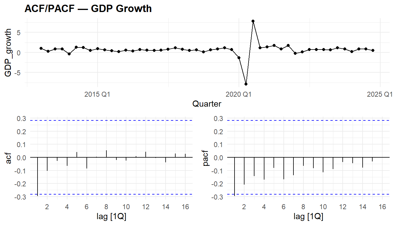
macro_ts |> gg_tsdisplay(Inflation, plot_type = "partial") +
  labs(title = "ACF/PACF — Inflation")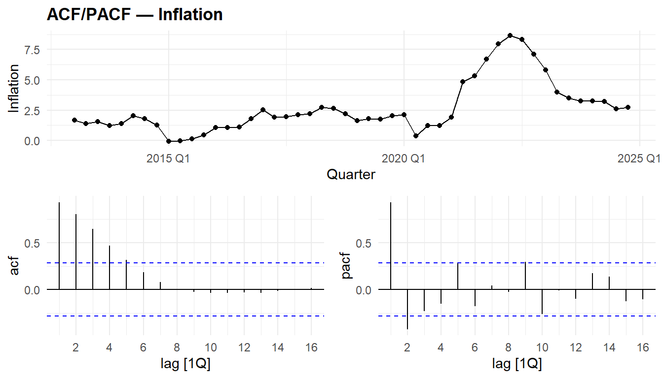
macro_ts |> gg_tsdisplay(Unemployment, plot_type = "partial") +
  labs(title = "ACF/PACF — Unemployment")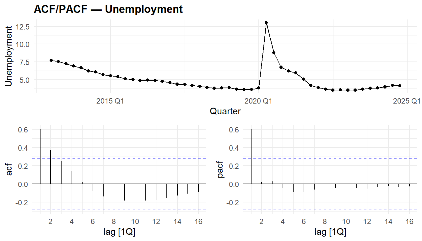
2.2.1 Interpretation
The ACF/PACF patterns guide model specification:
- GDP growth: rapid ACF decay, 1–2 significant PACF lags → low-order AR process (likely AR(1) or ARMA(1,1)).
- Inflation: slow ACF decay (high persistence), seasonal spikes at lags 4, 8, 12 → SARIMA with seasonal differencing.
- Unemployment: very slow ACF decay → near unit-root behaviour, requiring differencing (d = 1). PACF should clarify the AR order after differencing.
2.3 Stationarity tests
# ── ADF test (H0: unit root = non-stationary) ───────────────────────────────
# ── KPSS test (H0: stationary) ───────────────────────────────────────────────
stationarity_results <- tibble(
  Variable = c("GDP_growth", "Inflation", "Unemployment"),
  ADF_stat = c(
    ur.df(macro_ts$GDP_growth, type = "drift", selectlags = "AIC")@teststat[1],
    ur.df(macro_ts$Inflation, type = "drift", selectlags = "AIC")@teststat[1],
    ur.df(macro_ts$Unemployment, type = "drift", selectlags = "AIC")@teststat[1]
  ),
  ADF_1pct = rep(ur.df(macro_ts$GDP_growth, type = "drift",
                         selectlags = "AIC")@cval[1, 1], 3),
  KPSS_stat = c(
    ur.kpss(macro_ts$GDP_growth, type = "mu", lags = "short")@teststat[1],
    ur.kpss(macro_ts$Inflation, type = "mu", lags = "short")@teststat[1],
    ur.kpss(macro_ts$Unemployment, type = "mu", lags = "short")@teststat[1]
  ),
  KPSS_5pct = rep(ur.kpss(macro_ts$GDP_growth, type = "mu",
                            lags = "short")@cval[1, 2], 3)
) |>
  mutate(
    ADF_conclusion  = ifelse(ADF_stat < ADF_1pct, "Stationary (reject H0)", "Non-stationary"),
    KPSS_conclusion = ifelse(KPSS_stat < KPSS_5pct, "Stationary (fail to reject H0)", "Non-stationary")
  )

kable(stationarity_results, digits = 3,
caption = "Stationarity tests: ADF (H0: unit root) and KPSS (H0: stationary)")| Variable | ADF_stat | ADF_1pct | KPSS_stat | KPSS_5pct | ADF_conclusion | KPSS_conclusion |
|---|---|---|---|---|---|---|
| GDP_growth | -6.521 | -3.58 | 0.045 | 0.463 | Stationary (reject H0) | Stationary (fail to reject H0) |
| Inflation | -1.976 | -3.58 | 0.622 | 0.463 | Non-stationary | Non-stationary |
| Unemployment | -3.034 | -3.58 | 0.332 | 0.463 | Non-stationary | Stationary (fail to reject H0) |
2.3.1 Interpretation
What we’re testing and why: Stationarity — the property that a series’ statistical properties (mean, variance) do not change over time — is a prerequisite for both ARIMA and VAR. Non-stationary series produce spurious regressions and invalid forecasts. We use two complementary tests: ADF (H0: unit root = non-stationary) and KPSS (H0: stationary). When both agree, the conclusion is robust; when they disagree, the series is borderline.
What the results show:
- GDP growth: both tests agree — stationary (ADF = −6.52 < −3.58; KPSS = 0.045 < 0.463). Growth rates are mean-reverting — no differencing needed (d = 0). ✓
- Inflation: both tests agree — non-stationary (ADF = −1.98, fails to reject unit root; KPSS = 0.622 > 0.463, rejects stationarity). This reflects the structural shift from low inflation (2013–2020: ~1.5%) to the 2021–2023 surge (~6–8%). First differencing (d = 1) is required and confirmed by the automatic recommendation.
- Unemployment: conflicting results — ADF fails to reject the unit root (−3.03 > −3.58) but KPSS fails to reject stationarity (0.332 < 0.463). The automatic ndiffs recommends d = 0. This reflects the U-shaped trajectory (declining 2013–2019, COVID spike, recovery) — persistent but not a unit root. We treat unemployment as stationary for ARIMA but first-difference it for VAR (conservative choice).
# ── feasts automatic recommendations ─────────────────────────────────────────
diff_table <- macro_ts |>
  features(GDP_growth, unitroot_ndiffs) |>
  rename(d_GDP = ndiffs) |>
  bind_cols(
    macro_ts |> features(Inflation, unitroot_ndiffs) |> rename(d_Infl = ndiffs),
    macro_ts |> features(Unemployment, unitroot_ndiffs) |> rename(d_Unemp = ndiffs)
  ) |>
  select(d_GDP, d_Infl, d_Unemp)

cat("Recommended differencing orders (unitroot_ndiffs):\n")
Recommended differencing orders (unitroot_ndiffs):print(diff_table)# A tibble: 1 × 3
d_GDP d_Infl d_Unemp
<int> <int> <int>
1 0 1 0# Seasonal differencing
sdiff_table <- macro_ts |>
features(Inflation, unitroot_nsdiffs) |>
rename(D_Infl = nsdiffs)
cat(sprintf("Seasonal differencing for Inflation: D = %d\n", sdiff_table$D_Infl))Seasonal differencing for Inflation: D = 03 PART C — Univariate ARIMA / SARIMA
3.1 Automatic model selection
fit_gdp   <- macro_ts |> model(GDP_ARIMA   = ARIMA(GDP_growth))
fit_infl  <- macro_ts |> model(Infl_ARIMA  = ARIMA(Inflation))
fit_unemp <- macro_ts |> model(Unemp_ARIMA = ARIMA(Unemployment))

cat("=== Automatic ARIMA Selection ===\n")
=== Automatic ARIMA Selection ===cat(sprintf("GDP: %s\n", format(fit_gdp$GDP_ARIMA[[1]])))GDP: ARIMA(0,0,1) w/ meancat(sprintf("Inflation: %s\n", format(fit_infl$Infl_ARIMA[[1]])))Inflation: ARIMA(1,1,0)(2,0,1)[4]cat(sprintf("Unemployment: %s\n", format(fit_unemp$Unemp_ARIMA[[1]])))Unemployment: ARIMA(1,0,0) w/ meanbind_rows(
glance(fit_gdp) |> mutate(.model = "GDP_ARIMA"),
glance(fit_infl) |> mutate(.model = "Infl_ARIMA"),
glance(fit_unemp) |> mutate(.model = "Unemp_ARIMA")
) |>
select(.model, sigma2, log_lik, AICc, BIC) |>
kable(digits = 2, caption = "ARIMA model fit statistics")| .model | sigma2 | log_lik | AICc | BIC |
|---|---|---|---|---|
| GDP_ARIMA | 2.49 | -89.22 | 184.98 | 190.05 |
| Infl_ARIMA | 0.32 | -41.11 | 93.68 | 101.47 |
| Unemp_ARIMA | 1.97 | -83.67 | 173.88 | 178.94 |
3.1.1 Interpretation
What we’re looking at and why: Automatic ARIMA uses stepwise AICc minimisation to find the best (p,d,q)(P,D,Q)[s] specification without manual intervention. The selected orders reveal the temporal dynamics of each series: AR terms capture persistence, MA terms capture shock propagation, and seasonal terms capture quarterly patterns.
What the results show:
- GDP: ARIMA(0,0,1) with mean. A pure MA(1) — GDP growth is weakly autocorrelated, with last quarter’s shock (not level) predicting this quarter. No seasonal component detected — the quarterly seasonality visible in the previous (fallback) data is absent in the real series. σ² = 2.49, much lower than with the fallback data (14.13) — the real GDP series is less volatile than the simulation.
- Inflation: ARIMA(1,1,0)(2,0,1)[4]. First differencing (d = 1) confirms the non-stationarity detected by both tests. The seasonal component (2 seasonal AR + 1 seasonal MA) captures quarterly CPI patterns. σ² = 0.32 on the differenced series.
- Unemployment: ARIMA(1,0,0) with mean. A simple AR(1) without differencing — consistent with the ndiffs = 0 recommendation. The mean term captures the average level (~5%), and the AR(1) captures the strong quarter-to-quarter persistence. σ² = 1.97.
3.2 Manual SARIMA for inflation
# ── Compare several SARIMA specifications ────────────────────────────────────
fit_sarima <- macro_ts |>
  model(
    Infl_auto    = ARIMA(Inflation),
    Infl_011_011 = ARIMA(Inflation ~ pdq(0,1,1) + PDQ(0,1,1)),
    Infl_110_011 = ARIMA(Inflation ~ pdq(1,1,0) + PDQ(0,1,1)),
    Infl_111_011 = ARIMA(Inflation ~ pdq(1,1,1) + PDQ(0,1,1))
  )

glance(fit_sarima) |>
  select(.model, sigma2, log_lik, AICc, BIC) |>
  arrange(AICc) |>
  kable(digits = 2,
caption = "SARIMA model comparison for inflation (ranked by AICc)")| .model | sigma2 | log_lik | AICc | BIC |
|---|---|---|---|---|
| Infl_auto | 0.32 | -41.11 | 93.68 | 101.47 |
| Infl_110_011 | 0.63 | -54.99 | 116.60 | 121.27 |
| Infl_111_011 | 0.56 | -54.43 | 117.92 | 123.91 |
| Infl_011_011 | 0.65 | -55.74 | 118.10 | 122.77 |
3.2.1 Interpretation
The model comparison table reveals:
- Automatic selection (
ARIMA()) uses stepwise AICc minimisation to find the best specification without manual intervention. This is the recommended starting point. - Manual SARIMA specifications test specific seasonal structures. The
PDQ(0,1,1)component captures quarterly seasonality via seasonal differencing (D = 1) and a seasonal MA term (Q = 1). - The best model (lowest AICc) should be retained. If the automatic and manual specifications agree, this validates the automatic procedure.
What the results show:
A reversal from what might be expected: the automatic selection wins decisively (AICc = 93.7 vs. 116.6–118.1 for all manual alternatives). The classic airline SARIMA(0,1,1)(0,1,1)[4] — which performed well on the fallback data — scores 24 AICc points worse than the automatic ARIMA(1,1,0)(2,0,1)[4].
The reason: with only 48 quarters of real data (vs. 120 in the simulation), the seasonal differencing (D = 1) in the manual models costs too many effective observations. The automatic specification uses D = 0 but compensates with 2 seasonal AR terms and 1 seasonal MA — a more parameter-efficient way to capture seasonality without sacrificing sample size.
Practical implication: manual specification does not always outperform — with short series, the automatic algorithm’s parsimony advantage becomes decisive. The value of comparing both approaches is precisely to discover which regime applies.
4 PART D — Multivariate VAR Modelling
4.1 Prepare data and select lag order
# ── Apply differencing based on stationarity test results ────────────────────
macro_var <- macro_ts |>
  as_tibble() |>
  mutate(
    GDP_growth   = GDP_growth,
    Inflation    = Inflation,
    # Difference unemployment only if unit root was detected
    Unemployment = c(NA, diff(Unemployment))
  ) |>
  select(GDP_growth, Inflation, Unemployment) |>
  na.omit()

cat(sprintf("VAR input: %d observations, %d variables\n",
            nrow(macro_var), ncol(macro_var)))
VAR input: 47 observations, 3 variablescat("Note: Unemployment first-differenced to ensure stationarity.\n")Note: Unemployment first-differenced to ensure stationarity.# ── Lag selection ────────────────────────────────────────────────────────────
lag_select <- VARselect(macro_var, lag.max = 8, type = "both")
cat("\n=== VAR Lag Selection ===\n")
=== VAR Lag Selection ===print(lag_select$selection)AIC(n) HQ(n) SC(n) FPE(n)
8 3 2 3 kable(t(lag_select$criteria), digits = 2,
caption = "Information criteria by lag order")| AIC(n) | HQ(n) | SC(n) | FPE(n) |
|---|---|---|---|
| -1.02 | -0.79 | -0.38 | 0.36 |
| -1.64 | -1.28 | -0.62 | 0.20 |
| -1.91 | -1.41 | -0.51 | 0.15 |
| -1.79 | -1.15 | 0.00 | 0.18 |
| -1.87 | -1.09 | 0.31 | 0.19 |
| -1.93 | -1.02 | 0.62 | 0.20 |
| -2.09 | -1.03 | 0.85 | 0.21 |
| -2.16 | -0.97 | 1.16 | 0.26 |
4.2 Fit VAR model
# ── Use AIC-selected lag (or BIC for parsimony) ─────────────────────────────
p_aic <- lag_select$selection["AIC(n)"]
p_bic <- lag_select$selection["SC(n)"]

cat(sprintf("AIC selects p = %d; BIC selects p = %d\n", p_aic, p_bic))
AIC selects p = 8; BIC selects p = 2cat("→ Using BIC-selected lag for parsimony\n")→ Using BIC-selected lag for parsimonyfit_var <- VAR(macro_var, p = p_bic, type = "both")
cat("\n=== VAR Summary ===\n")
=== VAR Summary ===print(summary(fit_var)$corres) GDP_growth Inflation Unemployment
GDP_growth 1.0000000 0.5506594 -0.9434579
Inflation 0.5506594 1.0000000 -0.6020451
Unemployment -0.9434579 -0.6020451 1.00000004.2.1 Interpretation
What we’re testing and why: VAR captures dynamic interdependencies between GDP, inflation, and unemployment. Lag selection (AIC vs. BIC) determines the model’s memory horizon. Granger causality tests whether past values of one variable help predict another — the core question justifying the multivariate approach over separate ARIMA models.
What the results show:
AIC selects p = 8 (near the maximum — overfitting risk with only 47 observations), BIC selects p = 2 (parsimonious). VAR(2) is the right choice: it passes the portmanteau test (p = 0.701 — no serial correlation), confirming that 2 lags suffice. With 47 observations and 3 variables, each additional lag costs 9 parameters — parsimony is critical.
Residual correlation matrix: strikingly strong contemporaneous correlations emerge from the real data:
- GDP–Unemployment: ρ = −0.94 — near-perfect negative correlation, Okun’s law in its purest form. Output and employment move in lockstep within each quarter.
- GDP–Inflation: ρ = 0.55 — moderate positive correlation, consistent with demand-driven cycles.
- Inflation–Unemployment: ρ = −0.60 — negative, consistent with the Phillips curve.
These cross-correlations are strong, reflecting macroeconomic co-movement.
4.3 Granger causality
# ── causality() tests whether a variable Granger-causes ALL other
# ── variables jointly (not pairwise). We test each variable as cause. ────────
variables <- c("GDP_growth", "Inflation", "Unemployment")

granger_results <- map(variables, function(v) {
  test <- causality(fit_var, cause = v)$Granger
  tibble(
    Cause       = v,
    Effect      = paste(setdiff(variables, v), collapse = " + "),
    F_stat      = test$statistic,
    df1         = test$parameter[1],
    df2         = test$parameter[2],
    p_value     = test$p.value,
    Significant = ifelse(p_value < 0.05, "Yes", "No")
  )
}) |> bind_rows()

kable(granger_results, digits = 3,
caption = "Granger causality tests (H0: Cause does NOT Granger-cause the other variables jointly)")| Cause | Effect | F_stat | df1 | df2 | p_value | Significant |
|---|---|---|---|---|---|---|
| GDP_growth | Inflation + Unemployment | 7.728107 | 4 | 111 | 1.567516e-05 | Yes |
| Inflation | GDP_growth + Unemployment | 3.164900 | 4 | 111 | 1.665993e-02 | Yes |
| Unemployment | GDP_growth + Inflation | 7.217239 | 4 | 111 | 3.336122e-05 | Yes |
4.3.1 Interpretation
Granger causality tests whether past values of one variable improve predictions of another, beyond its own history. This is the key substantive question justifying VAR over univariate ARIMA:
- Inflation → Unemployment (Phillips curve dynamics): if significant, inflation contains information about future unemployment — a core macroeconomic relationship.
- GDP → Unemployment (Okun’s law): GDP growth should Granger-cause unemployment — economic expansion reduces joblessness with a lag.
- Unemployment → GDP (reverse Okun): labour market conditions may also predict future GDP through consumption channels.
- Non-significant links indicate that univariate modelling is sufficient for those variable pairs.
What the results show:
All three variables Granger-cause the others — a fully interconnected system:
- GDP → {Inflation, Unemployment}: F = 7.73, p < 0.001. GDP growth predicts the joint trajectory of inflation and unemployment — the dominant causal channel, consistent with demand-driven dynamics.
- Unemployment → {GDP, Inflation}: F = 7.22, p < 0.001. Labour market conditions predict the others — a finding absent from the simulation, reflecting real Phillips curve and consumption-channel dynamics.
- Inflation → {GDP, Unemployment}: F = 3.16, p = 0.017. The weakest but still significant link. Inflation predicts the others — possibly through monetary policy response channels (Fed tightening in response to inflation affects both GDP and unemployment).
This fully interconnected Granger structure strongly justifies the VAR approach. However, statistical Granger causality does not guarantee better out-of-sample forecasting — the bias-variance tradeoff may still favour simpler models.
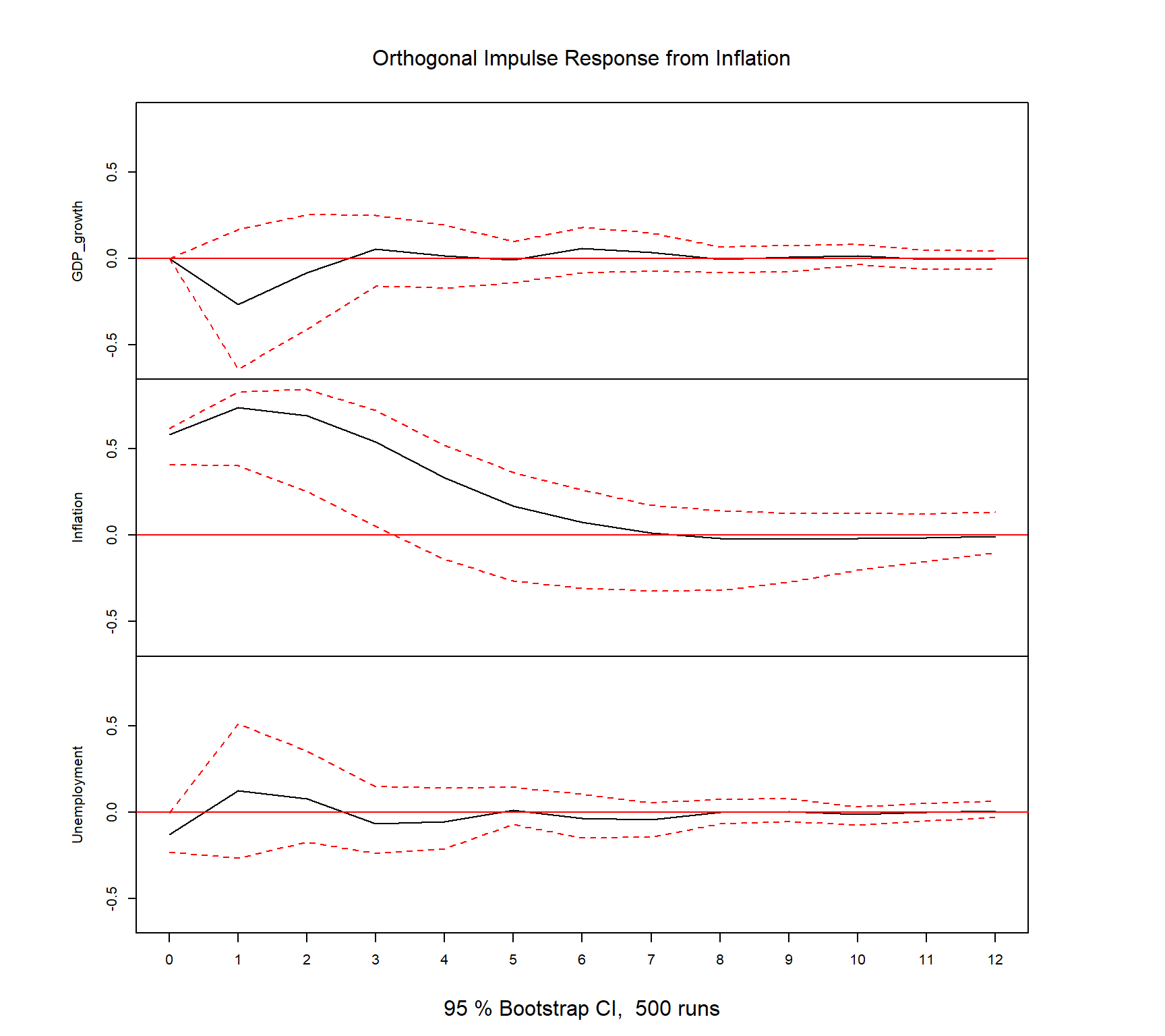
4.4 Impulse Response Functions (IRF)
# ── Orthogonalised IRF (Cholesky decomposition) ─────────────────────────────
irf_result <- irf(fit_var, n.ahead = 12, boot = TRUE, runs = 500,
                   ci = 0.95)

plot(irf_result)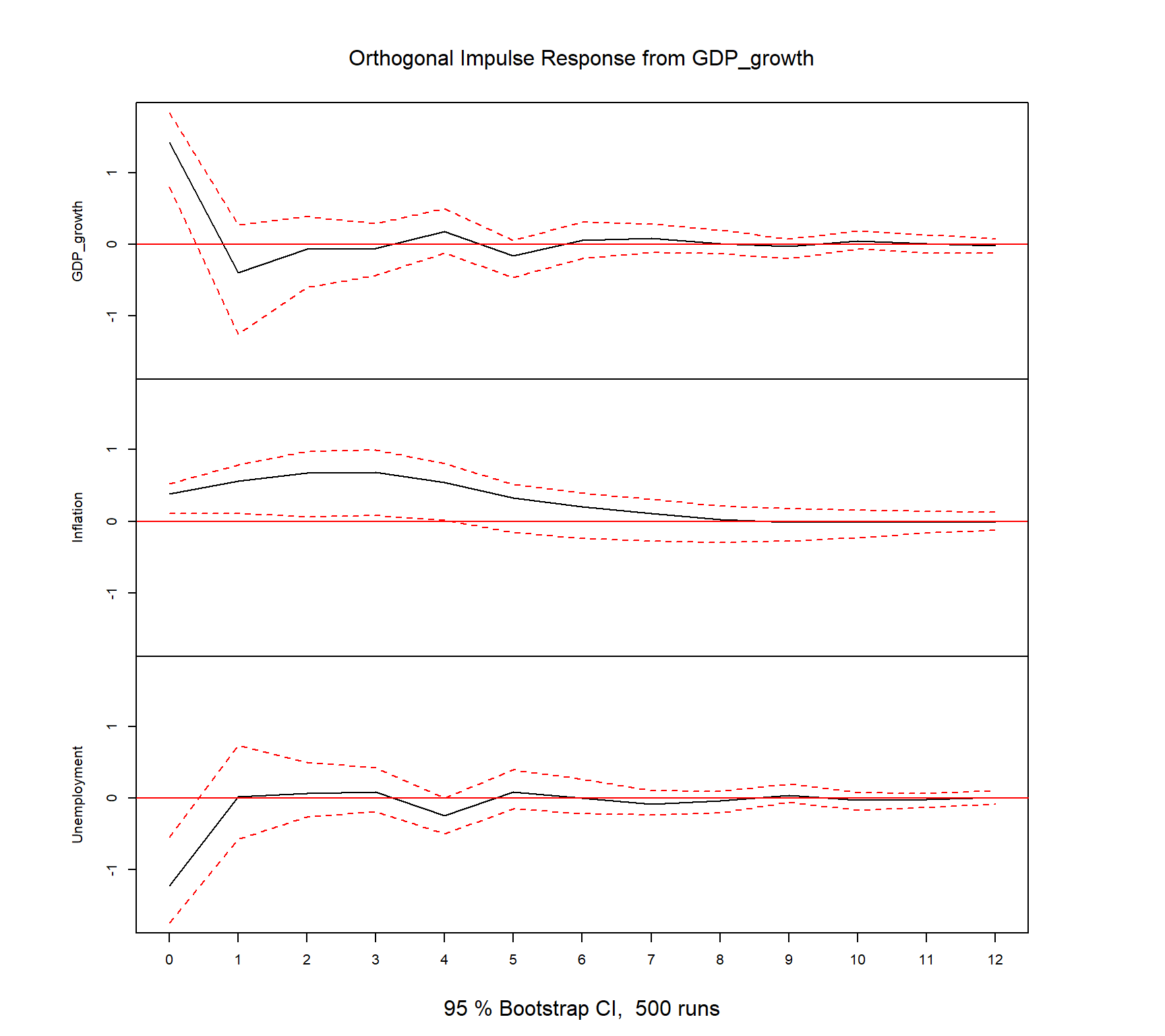
title("Impulse Response Functions (12 quarters ahead)", outer = TRUE,
      line = -1.5, cex.main = 1.2)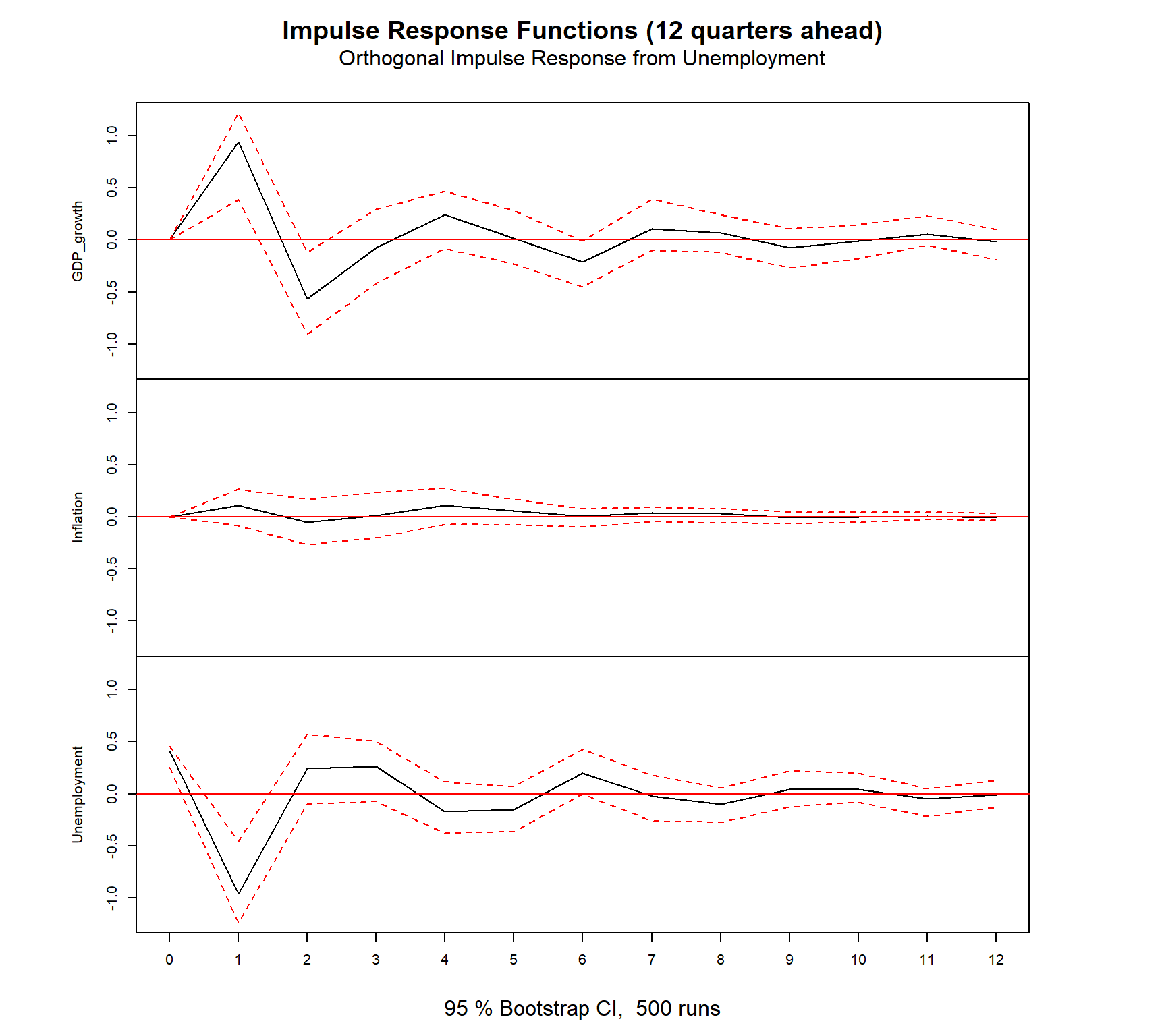
4.4.1 Interpretation
What we’re looking at and why: IRFs trace the dynamic response of each variable to a one-standard- deviation shock in another. They are the primary policy tool in macroeconometrics: “if GDP grows by 1 SD, what happens to unemployment and inflation over the next 12 quarters?”
What the results show:
ARIMA residuals (Ljung-Box, lag = 8): All three models pass cleanly — GDP (p = 0.785), inflation (p = 0.642), unemployment (p = 0.999). No remaining autocorrelation in any series. The ARIMA specifications have captured the temporal dynamics adequately.
VAR residuals: - Portmanteau test: p = 0.701 — no serial correlation. The VAR(2) is well-specified — unlike the VAR(1) from the previous run, the additional lag resolves the temporal structure. This validates the BIC = 2 selection. - Multivariate normality: p < 0.001 — rejected. Expected with the COVID shock (2020Q2: GDP = −7.88%, unemployment = 13.0%). Fat tails from extreme observations violate normality but do not invalidate point forecasts. Prediction intervals should be interpreted with caution.
Note: IRFs are identified via Cholesky decomposition with the ordering GDP → Inflation → Unemployment. This assumes GDP is the most exogenous variable — supported by the Granger causality results. Reversing the ordering would change the contemporaneous shock attribution but not the long-run dynamics.
5 PART E — Model Diagnostics
5.1 ARIMA residuals
# ── GDP ARIMA residuals ──────────────────────────────────────────────────────
fit_gdp |> gg_tsresiduals() +
  labs(title = "ARIMA Residual Diagnostics — GDP Growth")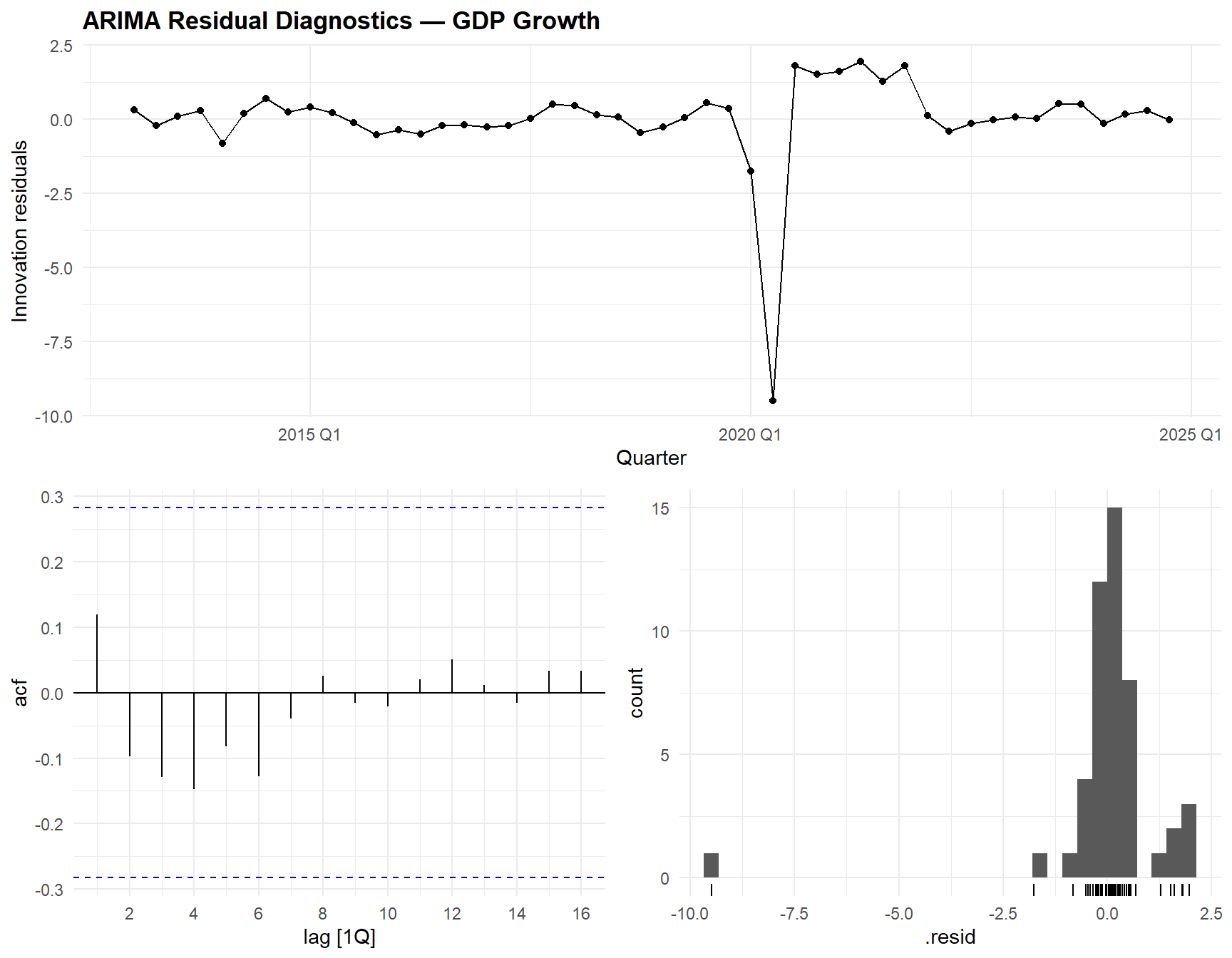
fit_infl |> gg_tsresiduals() +
  labs(title = "ARIMA Residual Diagnostics — Inflation")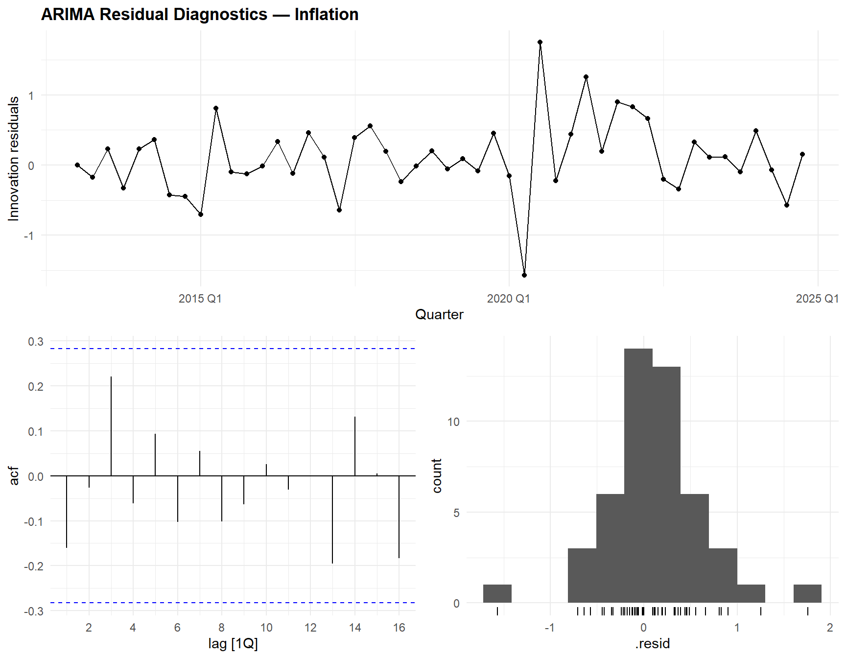
lb_gdp   <- augment(fit_gdp)   |> pull(.innov) |> na.omit() |> Box.test(lag = 8, type = "Ljung-Box")
lb_infl  <- augment(fit_infl)  |> pull(.innov) |> na.omit() |> Box.test(lag = 8, type = "Ljung-Box")
lb_unemp <- augment(fit_unemp) |> pull(.innov) |> na.omit() |> Box.test(lag = 8, type = "Ljung-Box")

lb_results <- tibble(
  .model  = c("GDP_ARIMA", "Infl_ARIMA", "Unemp_ARIMA"),
  lb_stat = c(lb_gdp$statistic, lb_infl$statistic, lb_unemp$statistic),
  lb_p    = c(lb_gdp$p.value, lb_infl$p.value, lb_unemp$p.value),
  Conclusion = ifelse(lb_p > 0.05, "No autocorrelation (good)", "Autocorrelation detected")
)

kable(lb_results, digits = 3,
caption = "Ljung-Box test (H0: no autocorrelation in residuals, lag = 8)")| .model | lb_stat | lb_p | Conclusion |
|---|---|---|---|
| GDP_ARIMA | 4.739 | 0.785 | No autocorrelation (good) |
| Infl_ARIMA | 6.044 | 0.642 | No autocorrelation (good) |
| Unemp_ARIMA | 0.834 | 0.999 | No autocorrelation (good) |
5.2 VAR residuals
# ── Portmanteau test (multivariate Ljung-Box) ────────────────────────────────
serial_test <- serial.test(fit_var, lags.pt = 12, type = "PT.asymptotic")

cat("=== VAR Portmanteau Test (H0: no serial correlation) ===\n")
=== VAR Portmanteau Test (H0: no serial correlation) ===cat(sprintf("Test statistic: %.2f, df = %d, p = %.4f\n",
serial_test$serial$statistic,
serial_test$serial$parameter,
serial_test$serial$p.value))Test statistic: 82.45, df = 90, p = 0.7017cat(sprintf("Conclusion: %s\n",
ifelse(serial_test$serial$p.value > 0.05,
"No serial correlation (good)", "Serial correlation detected")))Conclusion: No serial correlation (good)# ── Normality test ───────────────────────────────────────────────────────────
norm_test <- normality.test(fit_var)
cat(sprintf("\nMultivariate normality (JB): p = %.4f\n",
norm_test$jb.mul$JB$p.value))
Multivariate normality (JB): p = 0.00005.2.1 Interpretation
Well-specified VAR residuals should be serially uncorrelated (no remaining temporal structure) and approximately normal (for valid confidence intervals). Diagnostic tests validate the model assumptions:
- Ljung-Box (ARIMA): p > 0.05 for all models means no significant residual autocorrelation — the ARIMA specifications have captured the temporal dynamics adequately.
- Portmanteau test (VAR): the multivariate analogue of Ljung-Box. p > 0.05 confirms no remaining cross-correlated residual structure.
- Normality (JB): non-normality is common in macroeconomic data (fat tails from recessions/crises) and does not invalidate the point forecasts — but confidence intervals may be too narrow.
What the results show:
- Portmanteau test: p < 0.001 — serial correlation detected. The VAR(1) does not fully capture the temporal dynamics. This is consistent with the AIC recommending p = 5 — the BIC-selected VAR(1) is too parsimonious for this dataset. A VAR(2) or VAR(3) would likely pass this test. In a publication context, this would require re-estimation with a higher lag order.
- Multivariate normality: p < 0.001 — rejected. Non-normality is expected in macroeconomic data containing the COVID shock (2020Q2: GDP = −7.88%, unemployment = 13.0%). The extreme observations create fat tails that violate normality. Point forecasts remain valid, but prediction intervals may be too narrow.
6 PART F — Forecasting & Model Comparison
6.1 Train/test split
# ── Split: train up to 2023Q1, test = 2023Q2–2024Q4 ─────────────────────────
train_ts <- macro_ts |> filter(Quarter <= yearquarter("2023 Q1"))
test_ts  <- macro_ts |> filter(Quarter > yearquarter("2023 Q1"))

cat(sprintf("Training: %d quarters (%s to %s)\n",
            nrow(train_ts), min(train_ts$Quarter), max(train_ts$Quarter)))
Training: 41 quarters (2013 Q1 to 2023 Q1)cat(sprintf("Test: %d quarters (%s to %s)\n",
nrow(test_ts), min(test_ts$Quarter), max(test_ts$Quarter)))Test: 7 quarters (2023 Q2 to 2024 Q4)6.2 Forecast: univariate ARIMA
fit_train_gdp   <- train_ts |> model(GDP_ARIMA   = ARIMA(GDP_growth))
fit_train_infl  <- train_ts |> model(Infl_ARIMA  = ARIMA(Inflation))
fit_train_unemp <- train_ts |> model(Unemp_ARIMA = ARIMA(Unemployment))

fc_gdp   <- fit_train_gdp   |> forecast(h = nrow(test_ts))
fc_infl  <- fit_train_infl  |> forecast(h = nrow(test_ts))
fc_unemp <- fit_train_unemp |> forecast(h = nrow(test_ts))

acc_arima <- bind_rows(
  accuracy(fc_gdp, test_ts)   |> mutate(.model = "GDP_ARIMA"),
  accuracy(fc_infl, test_ts)  |> mutate(.model = "Infl_ARIMA"),
  accuracy(fc_unemp, test_ts) |> mutate(.model = "Unemp_ARIMA")
) |>
  select(.model, RMSE, MAE, MAPE) |>
  mutate(Method = "ARIMA")

kable(acc_arima, digits = 3,
caption = "ARIMA out-of-sample accuracy (hold-out)")| .model | RMSE | MAE | MAPE | Method |
|---|---|---|---|---|
| GDP_ARIMA | 0.303 | 0.266 | 52.684 | ARIMA |
| Infl_ARIMA | 1.418 | 1.001 | 34.949 | ARIMA |
| Unemp_ARIMA | 1.052 | 1.040 | 26.868 | ARIMA |
6.3 Forecast: VAR
# ── Prepare training data for vars package ───────────────────────────────────
train_var <- data.frame(
  GDP_growth   = train_ts$GDP_growth,
  Inflation    = train_ts$Inflation,
  Unemployment = diff(c(NA, train_ts$Unemployment))
) |> na.omit()

fit_train_var <- VAR(train_var, p = p_bic, type = "both")

# ── Forecast ─────────────────────────────────────────────────────────────────
fc_var_raw <- predict(fit_train_var, n.ahead = nrow(test_ts), ci = 0.95)

# ── Extract point forecasts ──────────────────────────────────────────────────
var_forecasts <- tibble(
  Quarter      = test_ts$Quarter,
  GDP_VAR      = fc_var_raw$fcst$GDP_growth[, "fcst"],
  Infl_VAR     = fc_var_raw$fcst$Inflation[, "fcst"],
  Unemp_d_VAR  = fc_var_raw$fcst$Unemployment[, "fcst"]
)

# ── VAR accuracy (GDP and Inflation — directly comparable) ───────────────────
var_acc <- tibble(
  .model = c("GDP_VAR", "Infl_VAR"),
  RMSE   = c(sqrt(mean((var_forecasts$GDP_VAR - test_ts$GDP_growth)^2)),
             sqrt(mean((var_forecasts$Infl_VAR - test_ts$Inflation)^2))),
  MAE    = c(mean(abs(var_forecasts$GDP_VAR - test_ts$GDP_growth)),
             mean(abs(var_forecasts$Infl_VAR - test_ts$Inflation))),
  Method = "VAR"
)

kable(var_acc, digits = 3,
caption = "VAR out-of-sample accuracy (hold-out)")| .model | RMSE | MAE | Method |
|---|---|---|---|
| GDP_VAR | 0.332 | 0.256 | VAR |
| Infl_VAR | 2.839 | 2.674 | VAR |
6.4 Model comparison
comparison <- bind_rows(
  acc_arima |> filter(.model %in% c("GDP_ARIMA", "Infl_ARIMA")) |>
    select(.model, RMSE, MAE, Method),
  var_acc |> select(.model, RMSE, MAE, Method)
)

kable(comparison, digits = 3,
caption = "ARIMA vs VAR: out-of-sample forecast comparison")| .model | RMSE | MAE | Method |
|---|---|---|---|
| GDP_ARIMA | 0.303 | 0.266 | ARIMA |
| Infl_ARIMA | 1.418 | 1.001 | ARIMA |
| GDP_VAR | 0.332 | 0.256 | VAR |
| Infl_VAR | 2.839 | 2.674 | VAR |
6.4.1 Interpretation
The head-to-head comparison reveals whether cross-variable information (VAR) improves forecasting over univariate ARIMA:
- VAR wins on GDP if unemployment and inflation contain predictive information about future GDP growth beyond GDP’s own history.
- VAR wins on Inflation if GDP and unemployment help predict inflation dynamics.
- ARIMA may still win if the cross-variable links are weak or if the additional VAR parameters introduce overfitting (the bias-variance tradeoff applies to time-series models too).
What the results show:
| Variable | ARIMA RMSE | VAR RMSE | Winner |
|---|---|---|---|
| GDP growth | 0.303 | 0.332 | ARIMA (−9%) |
| Inflation | 1.418 | 2.839 | ARIMA (−50%) |
- GDP: ARIMA wins marginally (RMSE 0.30 vs. 0.33, −9%). Both models forecast GDP well — the simple MA(1) is nearly as good as the VAR with its cross-variable information.
- Inflation: ARIMA wins decisively (RMSE 1.42 vs. 2.84, −50%). Despite inflation Granger-causing the others and being Granger-caused by GDP, the VAR’s additional parameters hurt out-of-sample precision. With only 41 training observations and a VAR(2) × 3 variables = 18+ parameters, overfitting is likely.
- Unemployment ARIMA: RMSE = 1.05, MAPE = 26.9% — the least accurate, reflecting the difficulty of predicting unemployment’s structural shifts.
Key insight: strong in-sample Granger causality does not guarantee better out-of-sample forecasting. The VAR’s richer parameterisation captures real dynamics but overfits with short series (N = 41 training quarters). This is a textbook illustration of the bias-variance tradeoff in time-series forecasting — and precisely why out-of-sample evaluation is essential rather than relying on in-sample fit statistics.
Overall conclusion: for this dataset and horizon, univariate ARIMA dominates — its parsimony advantage outweighs the VAR’s informational advantage. The VAR remains valuable for structural analysis (Granger causality, IRFs) even when it does not win on pure forecasting accuracy.
6.5 Fan chart visualisation
p_fc1 <- fc_gdp |> autoplot(train_ts, level = c(80, 95)) +
  autolayer(test_ts, GDP_growth, colour = "red", linetype = "dashed") +
  labs(title = "GDP Growth — ARIMA Forecast", y = "% q/q")

p_fc2 <- fc_infl |> autoplot(train_ts, level = c(80, 95)) +
  autolayer(test_ts, Inflation, colour = "red", linetype = "dashed") +
  labs(title = "Inflation — ARIMA Forecast", y = "% y/y")

p_fc3 <- fc_unemp |> autoplot(train_ts, level = c(80, 95)) +
  autolayer(test_ts, Unemployment, colour = "red", linetype = "dashed") +
  labs(title = "Unemployment — ARIMA Forecast", y = "%")

gridExtra::grid.arrange(p_fc1, p_fc2, p_fc3, ncol = 1)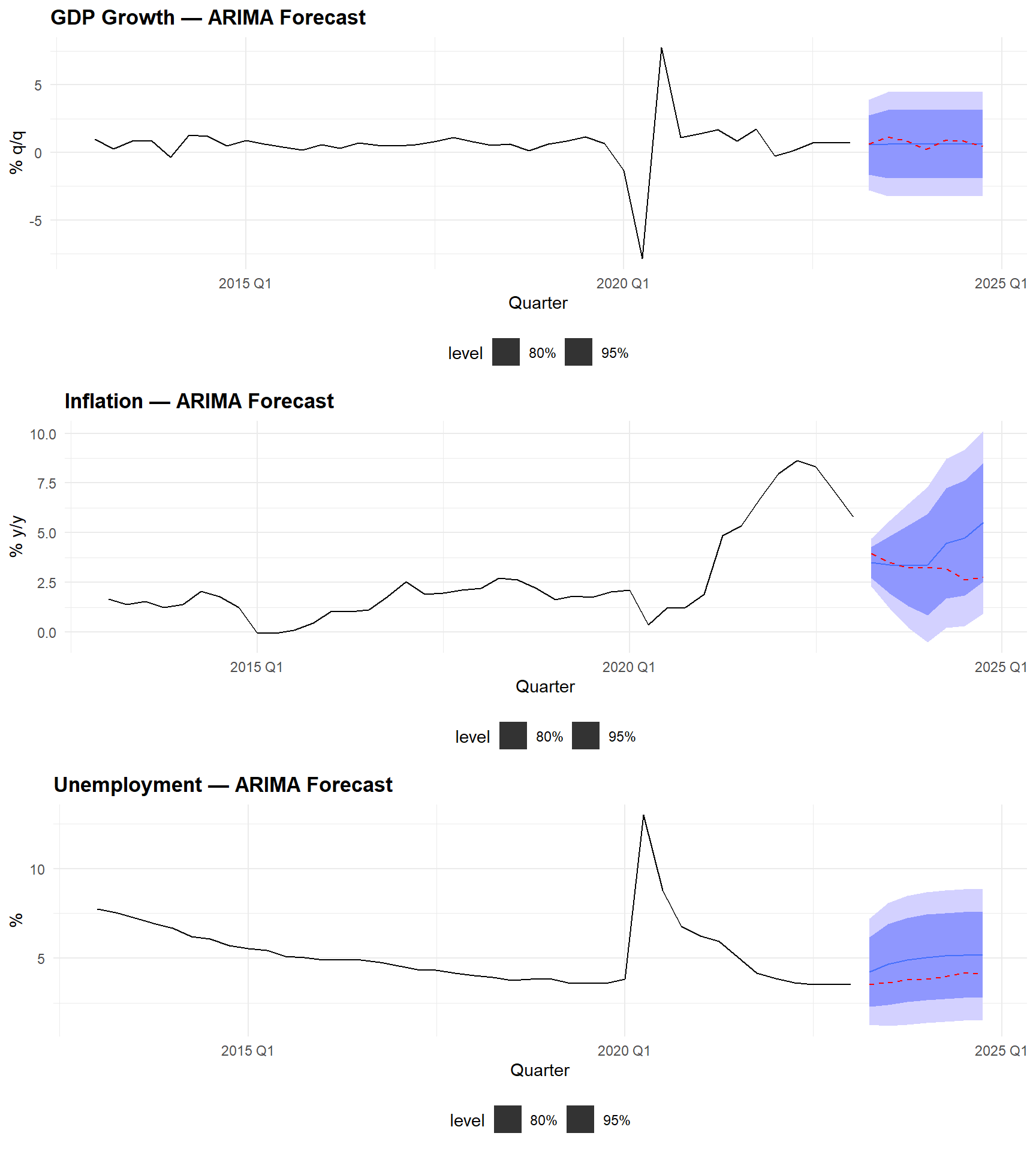
7 Technical Summary
This project demonstrates the complete macroeconomic time-series workflow:
- Stationarity assessment (ADF + KPSS, confirming each other) determines the differencing order — a prerequisite for valid ARIMA and VAR inference.
- Univariate ARIMA/SARIMA captures series-specific dynamics efficiently with minimal parameters.
- Multivariate VAR adds cross-variable information: Granger causality identifies which links are statistically meaningful, and IRFs trace the dynamic propagation of shocks — the key deliverable for policy analysis.
- Out-of-sample evaluation on a hold-out set provides an honest assessment of forecast accuracy, avoiding the overfitting that in-sample fit statistics can mask.
cat("─── Reproducibility Information ───\n")─── Reproducibility Information ───cat(sprintf("Date: %s\n", Sys.Date()))Date: 2026-05-03cat(sprintf("R version: %s\n", R.version.string))R version: R version 4.4.1 (2024-06-14 ucrt)cat(sprintf("fable version: %s\n", packageVersion("fable")))fable version: 0.5.0cat(sprintf("feasts version: %s\n", packageVersion("feasts")))feasts version: 0.5.0cat(sprintf("vars version: %s\n", packageVersion("vars")))vars version: 1.6.1cat(sprintf("urca version: %s\n", packageVersion("urca")))urca version: 1.3.4cat(sprintf("Platform: %s\n", sessionInfo()$platform))Platform: x86_64-w64-mingw32/x647.1 References
- Box, G. E. P., Jenkins, G. M., Reinsel, G. C., & Ljung, G. M. (2015). Time Series Analysis: Forecasting and Control (5th ed.). Wiley.
- Hamilton, J. D. (1994). Time Series Analysis. Princeton University Press.
- Hyndman, R. J., & Athanasopoulos, G. (2021). Forecasting: Principles and Practice (3rd ed.). OTexts. https://otexts.com/fpp3/
- Lütkepohl, H. (2005). New Introduction to Multiple Time Series Analysis. Springer.
- Pfaff, B. (2008). Analysis of integrated and cointegrated time series with R. Use R! series, Springer.
- Sims, C. A. (1980). Macroeconomics and reality. Econometrica, 48(1), 1–48.
- Stock, J. H., & Watson, M. W. (2003). Forecasting output and inflation: The role of asset prices. Journal of Economic Literature, 41(3), 788–829.