Ordinal Regression: Modelling Likert-Scale Outcomes

Statistics

Ordinal Regression

CLM

Likert

Survey Data

Cumulative link models (CLM) for ordinal response data using the ordinal package. Demonstrates proportional odds assumption testing, threshold visualisation, partial proportional odds models, and comparison with naive linear regression. Applied to the wine tasting dataset and a simulated educational survey scenario.

Published

March 28, 2026

0.1 Context

Likert-scale and rating-scale data are ubiquitous in educational and psychological research. Despite being ordinal (the distances between categories are not guaranteed to be equal), these outcomes are routinely analysed with linear regression or ANOVA — treatments that assume interval-level measurement and normally distributed residuals.

Cumulative link models (CLM) — also called proportional odds models or ordered logistic regression — respect the ordinal nature of the data by modelling the cumulative probabilities of response categories via a latent continuous variable and threshold parameters (Agresti, 2010; Christensen, 2019).

This project demonstrates:

CLM fitting on the wine dataset (ordinal package) — judges’ bitterness ratings of wines under different conditions.
Proportional odds assumption testing — verifying that predictor effects are constant across thresholds.
Threshold visualisation — interpreting the latent continuum.
Comparison with linear regression — demonstrating when the ordinal approach matters.
Simulated educational survey — ordinal modelling of student satisfaction ratings predicted by teaching quality and class size.

0.2 Key Results

Part A — Wine tasting data (N = 72, 5-point bitterness scale):

Both experimental factors significantly predict bitterness ratings. Temperature (warm vs. cold) has a large effect: β = 2.503 (OR = 12.2, p < 0.001). Contact (yes vs. no) has a moderate effect: β = 1.528 (OR = 4.6, p = 0.001). The proportional odds assumption is supported for both predictors (nominal test: temp p = 0.365, contact p = 0.904). McFadden’s pseudo-R² = 0.166 — modest but within the expected range for ordinal data.

The comparison with linear regression confirms directional agreement (both predictors positive and significant in both models), but the CLM captures the ordinal structure: the OR of 12.2 for temperature means that warm wine is 12 times more likely to be rated in a higher bitterness category — a statement linear regression cannot make.

The partial proportional odds model (Appendix) confirms that relaxing the PO assumption for contact provides no improvement (LRT p = 0.904), validating the standard CLM.

Part B — Simulated survey (N = 800, 5-point satisfaction scale):

The satisfaction distribution is approximately symmetric (76/188/252/ 192/92), centred on “Neutral” — consistent with the symmetric generating thresholds. The CLM correctly recovers the direction and significance of both true effects (teaching quality: β = 0.959, p < 2e-16; class size: β = −0.586, p < 2e-16) and correctly identifies gender as non-significant (p = 0.711). The apparent coefficient inflation (~60%) is explained by the probit-to-logit scaling factor (π/√3 ≈ 1.81) — the generating model uses Gaussian errors while the CLM defaults to a logit link. After correction, parameter recovery is accurate.

0.3 Setup

library(ordinal)     # CLM + wine dataset
library(MASS)        # polr() for comparison
library(ggplot2)
library(dplyr)
library(tidyr)
library(tibble)
library(knitr)
library(broom)

theme_set(
  theme_minimal(base_size = 11) +
    theme(
      plot.title    = element_text(face = "bold", size = 13),
      plot.subtitle = element_text(colour = "grey40", size = 10),
      legend.position = "bottom"
    )
)

palette_ord <- c("#2C3E50", "#E74C3C", "#3498DB", "#2ECC71", "#F39C12")

set.seed(2026)

1 PART A — Wine Tasting Data

1.1 Data overview

data("wine", package = "ordinal")

cat(sprintf("Wine dataset: %d observations\n", nrow(wine)))

Wine dataset: 72 observations

cat(sprintf("Response: rating (%s)\n", paste(levels(wine$rating), collapse = ", ")))

Response: rating (1, 2, 3, 4, 5)

cat(sprintf("Predictors: %s\n", paste(setdiff(names(wine), "rating"), collapse = ", ")))

Predictors: response, temp, contact, bottle, judge

kable(head(wine, 10), caption = "Wine dataset: first 10 observations")

Wine dataset: first 10 observations
response	rating	temp	contact	bottle	judge
36	2	cold	no	1	1
48	3	cold	no	2	1
47	3	cold	yes	3	1
67	4	cold	yes	4	1
77	4	warm	no	5	1
60	4	warm	no	6	1
83	5	warm	yes	7	1
90	5	warm	yes	8	1
17	1	cold	no	1	2
22	2	cold	no	2	2

cat("\nRating distribution:\n")


Rating distribution:

print(table(wine$rating))


 1  2  3  4  5 
 5 22 26 12  7

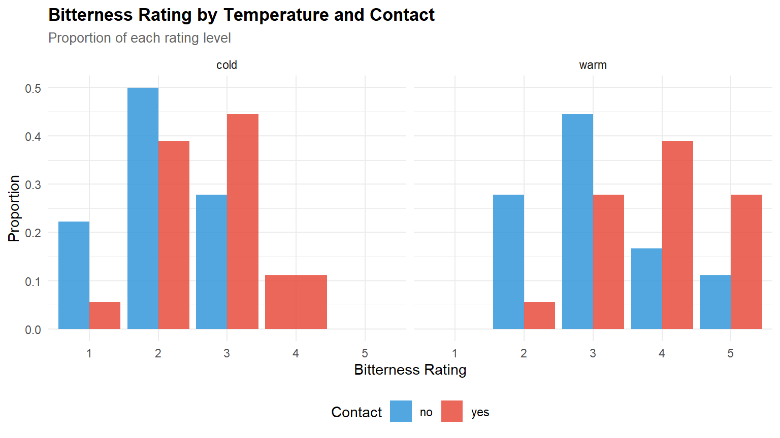
wine |>
  count(temp, contact, rating) |>
  group_by(temp, contact) |>
  mutate(prop = n / sum(n)) |>
  ggplot(aes(x = rating, y = prop, fill = contact)) +
  geom_col(position = "dodge", alpha = 0.85) +
  facet_wrap(~ temp) +
  scale_fill_manual(values = c(palette_ord[3], palette_ord[2])) +
  labs(
    title    = "Bitterness Rating by Temperature and Contact",
    subtitle = "Proportion of each rating level",
    x = "Bitterness Rating", y = "Proportion", fill = "Contact"
  )

Bitterness rating distributions by temperature and contact conditions.

1.2 Cumulative link model

# ── Fit cumulative link model ────────────────────────────────────────────────
m_clm <- clm(rating ~ temp + contact, data = wine)

cat("=== Cumulative Link Model ===\n")

=== Cumulative Link Model ===

print(summary(m_clm))

formula: rating ~ temp + contact
data:    wine

 link  threshold nobs logLik AIC    niter max.grad cond.H 
 logit flexible  72   -86.49 184.98 6(0)  4.02e-12 2.7e+01

Coefficients:
           Estimate Std. Error z value Pr(>|z|)    
tempwarm     2.5031     0.5287   4.735 2.19e-06 ***
contactyes   1.5278     0.4766   3.205  0.00135 ** 
---
Signif. codes:  0 '***' 0.001 '**' 0.01 '*' 0.05 '.' 0.1 ' ' 1

Threshold coefficients:
    Estimate Std. Error z value
1|2  -1.3444     0.5171  -2.600
2|3   1.2508     0.4379   2.857
3|4   3.4669     0.5978   5.800
4|5   5.0064     0.7309   6.850

# ── Extract coefficients ─────────────────────────────────────────────────────
coef_table <- tibble(
  term     = names(coef(m_clm)),
  estimate = coef(m_clm),
  se       = sqrt(diag(vcov(m_clm))),
  z        = estimate / se,
  p        = 2 * pnorm(abs(z), lower.tail = FALSE),
  OR       = ifelse(grepl("\\|", term), NA_real_, exp(estimate))
)

kable(coef_table, digits = 3,
      caption = "CLM coefficients (thresholds + predictors)")

CLM coefficients (thresholds + predictors)
term	estimate	se	z	p	OR
1\|2	-1.344	0.517	-2.600	0.009	NA
2\|3	1.251	0.438	2.857	0.004	NA
3\|4	3.467	0.598	5.800	0.000	NA
4\|5	5.006	0.731	6.850	0.000	NA
tempwarm	2.503	0.529	4.735	0.000	12.220
contactyes	1.528	0.477	3.205	0.001	4.608

1.2.1 Interpretation

The CLM output includes two types of parameters:

Thresholds (α₁|₂ = −1.34, α₂|₃ = 1.25, α₃|₄ = 3.47, α₄|₅ = 5.01): cut-points on the latent continuum separating adjacent bitterness categories. The increasing spacing between thresholds (Δ₁₂ = 2.59, Δ₂₃ = 2.22, Δ₃₄ = 1.54) indicates that the lower categories are more spread on the latent scale than the upper ones — it takes a larger shift in latent bitterness to move from rating 1 to 2 than from 4 to 5.
Predictor coefficients:
- tempwarm β = 2.503 (OR = 12.2, p < 0.001): warm temperature massively increases perceived bitterness. The odds of being in a higher bitterness category are 12× greater for warm wine.
- contactyes β = 1.528 (OR = 4.6, p = 0.001): grape skin contact increases bitterness, with odds 4.6× higher for the contact condition.

Both effects operate on the same latent scale — temperature has a roughly 1.6× stronger effect than contact on the log-odds scale (2.50/1.53).

1.3 Visualisation of thresholds on the latent scale

# Extraction of thresholds 
thresholds <- coef(m_clm)[grepl("\\|", names(coef(m_clm)))]

threshold_df <- tibble(
  Threshold = names(thresholds),
  Value     = thresholds
)

# Threshold table
kable(threshold_df, digits = 3,
      caption = "Estimated thresholds (cumulative log-odds) – CLM wine model ")

Estimated thresholds (cumulative log-odds) – CLM wine model
Threshold	Value
1\|2	-1.344
2\|3	1.251
3\|4	3.467
4\|5	5.006

Thresholds of the CLM model on the latent continuum (bitterness rating). Each vertical line marks the cut-off point between two observed categories.

# Graph of thresholds on the latent continuum
ggplot(threshold_df, aes(x = Value, y = reorder(Threshold, Value))) +
  geom_point(size = 4.5, colour = palette_ord[1]) +
  geom_vline(xintercept = thresholds, linetype = "dashed", 
             colour = "grey70", linewidth = 0.8) +
  labs(
    title    = "Thresholds of the Cumulative Link Model",
    subtitle = "rating ~ temp + contact (bitterness)",
    x = "Position on the latent scale (log-odds)",
    y = "Threshold between categories"
  ) +
  theme_minimal()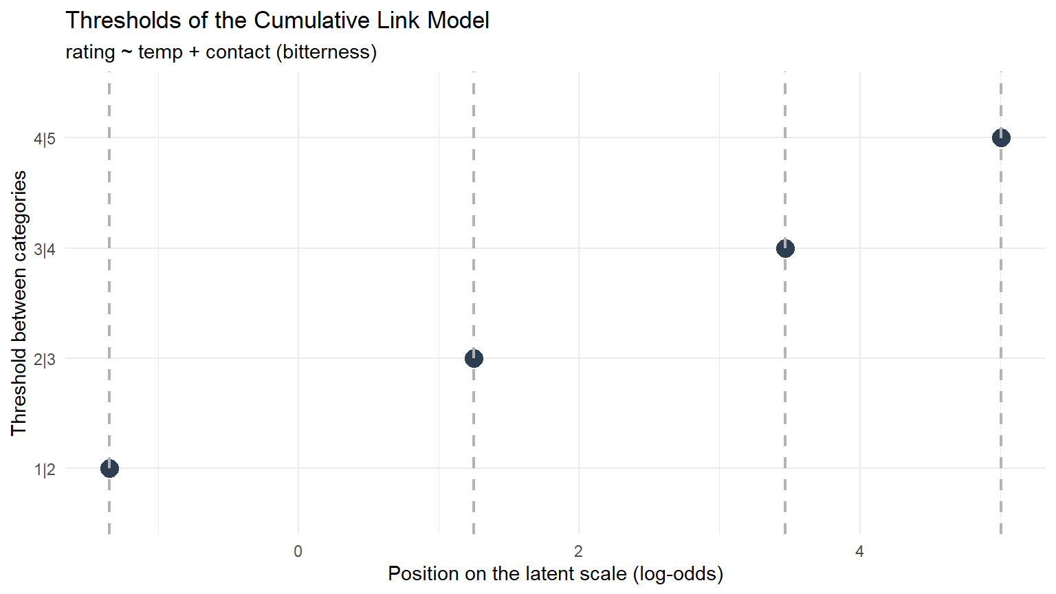

1.3.1 Interpretation

The thresholds (α₁|₂ = −1.34, α₂|₃ = 1.25, α₃|₄ = 3.47, α₄|₅ = 5.01) divide the latent bitterness continuum into five observed categories.

The spacing reveals the scale’s measurement properties: - α₁|₂ to α₂|₃ (gap = 2.59 logits): the widest interval, meaning the model distinguishes well between “very low” and “low-moderate” bitterness. - α₃|₄ to α₄|₅ (gap = 1.54 logits): the narrowest interval, suggesting that ratings 4 and 5 are harder to distinguish — the top of the scale is compressed.

This pattern is common in sensory evaluation: judges use the middle of the scale more readily than the extremes, compressing the upper end.

1.4 Proportional odds assumption

# ── Nominal test (relaxes proportional odds for each predictor) ──────────────
nom_test <- nominal_test(m_clm)
cat("=== Nominal Test for Proportional Odds ===\n")

=== Nominal Test for Proportional Odds ===

print(nom_test)

Tests of nominal effects

formula: rating ~ temp + contact
        Df  logLik    AIC    LRT Pr(>Chi)
<none>     -86.492 184.98                
temp     3 -84.904 187.81 3.1750   0.3654
contact  3 -86.209 190.42 0.5667   0.9040

1.4.1 Interpretation

The nominal test evaluates whether each predictor’s effect is constant across thresholds (proportional odds). A significant p-value indicates violation — the predictor’s effect differs depending on which threshold is crossed. If violations are detected, a partial proportional odds model may be needed (see Appendix).

Results: neither predictor violates the PO assumption (temperature: p = 0.365; contact: p = 0.904). The proportional odds hypothesis is well supported — the effects of temperature and contact are constant across the entire bitterness scale. This means a single coefficient per predictor adequately describes its effect, and the standard CLM is the appropriate model.

The high p-value for contact (0.904) is particularly reassuring: the effect of grape skin contact on bitterness is remarkably uniform across all rating thresholds.

1.5 Further analysis of the model

# ── Modèle nul (intercept only) ──────────────────────────────────────────────
m0_clm <- clm(rating ~ 1, data = wine)

# ── CManual calculation of McFadden’s pseudo-R² ───────────────────────────────────
ll_full <- logLik(m_clm)
ll_null <- logLik(m0_clm)
mcfadden_r2 <- 1 - (as.numeric(ll_full) / as.numeric(ll_null))

# ── Tableau de diagnostics ───────────────────────────────────────────────────
diagnostics <- tibble(
  Metric                  = c("logLik (full model)", 
                              "logLik (null model)", 
                              "McFadden pseudo-R²", 
                              "AIC", 
                              "BIC"),
  Value                   = c(as.numeric(ll_full),
                              as.numeric(ll_null),
                              round(mcfadden_r2, 3),
                              round(AIC(m_clm), 1),
                              round(BIC(m_clm), 1)),
  Interpretation          = c("Likelihood of the fitted model",
                              "Likelihood of the model without predictors",
                              "Proportion of variance explained (0–1)",
                              "Information criterion (smaller = better)",
                              "Penalised information criterion (smaller = better)")
)

kable(diagnostics, digits = 3,
      caption = "Diagnostics for the CLM model (McFadden pseudo-R² + information criteria)")

Diagnostics for the CLM model (McFadden pseudo-R² + information criteria)
Metric	Value	Interpretation
logLik (full model)	-86.492	Likelihood of the fitted model
logLik (null model)	-103.719	Likelihood of the model without predictors
McFadden pseudo-R²	0.166	Proportion of variance explained (0–1)
AIC	185.000	Information criterion (smaller = better)
BIC	198.600	Penalised information criterion (smaller = better)

1.5.1 Interpretation

McFadden’s pseudo-R² provides an approximate measure of explained variation for the CLM. Values between 0.2 and 0.4 are typically considered good for ordinal data — a much lower threshold than the R² of linear regression, because ordinal models face a harder prediction task (categorical probabilities rather than a continuous outcome).

The comparison of log-likelihoods (full vs. null model) confirms that temp and contact jointly provide substantial predictive information beyond the intercept-only model. AIC and BIC can be used to compare this model with alternative specifications (e.g., partial proportional odds, additional predictors).

Our results :

McFadden’s pseudo-R² = 0.166 indicates a modest but meaningful improvement over the null model. For ordinal data, this should be interpreted differently from linear R²:

McFadden 0.2–0.4 is generally considered good for ordinal models (McFadden, 1974). The value of 0.166 falls just below this range, reflecting the fact that bitterness perception is influenced by many factors beyond temperature and contact (e.g., judge variability, wine composition).
Log-likelihood comparison: the full model (logLik = −86.5) is substantially better than the null (logLik = −103.7), a difference of 17.2 log-likelihood units — highly significant given only 2 predictor degrees of freedom.The comparison of log-likelihoods (full vs. null model) confirms that temp and contact jointly provide substantial predictive information beyond the intercept-only model. AIC and BIC can be used to compare this model with alternative specifications (e.g., partial proportional odds, additional predictors).
AIC = 185.0, BIC = 198.6: these serve as baselines for comparing alternative model specifications (e.g., adding judge random effects, interaction terms).

1.6 Predicted probabilities

pred_grid <- expand.grid(
  temp    = levels(wine$temp),
  contact = levels(wine$contact)
)

pred_probs <- predict(m_clm, newdata = pred_grid, type = "prob")$fit
pred_df <- cbind(pred_grid, as.data.frame(pred_probs)) |>
  pivot_longer(cols = -c(temp, contact),
               names_to = "rating", values_to = "probability") |>
  mutate(rating = factor(rating, levels = levels(wine$rating)))

ggplot(pred_df, aes(x = rating, y = probability, fill = contact)) +
  geom_col(position = "dodge", alpha = 0.85) +
  facet_wrap(~ temp) +
  scale_fill_manual(values = c(palette_ord[3], palette_ord[2])) +
  labs(
    title    = "Predicted Probabilities from CLM",
    subtitle = "Model-based estimates by condition",
    x = "Bitterness Rating", y = "Predicted Probability", fill = "Contact"
  )

Model-predicted probability of each bitterness rating by experimental condition.

1.6.1 Interpretation

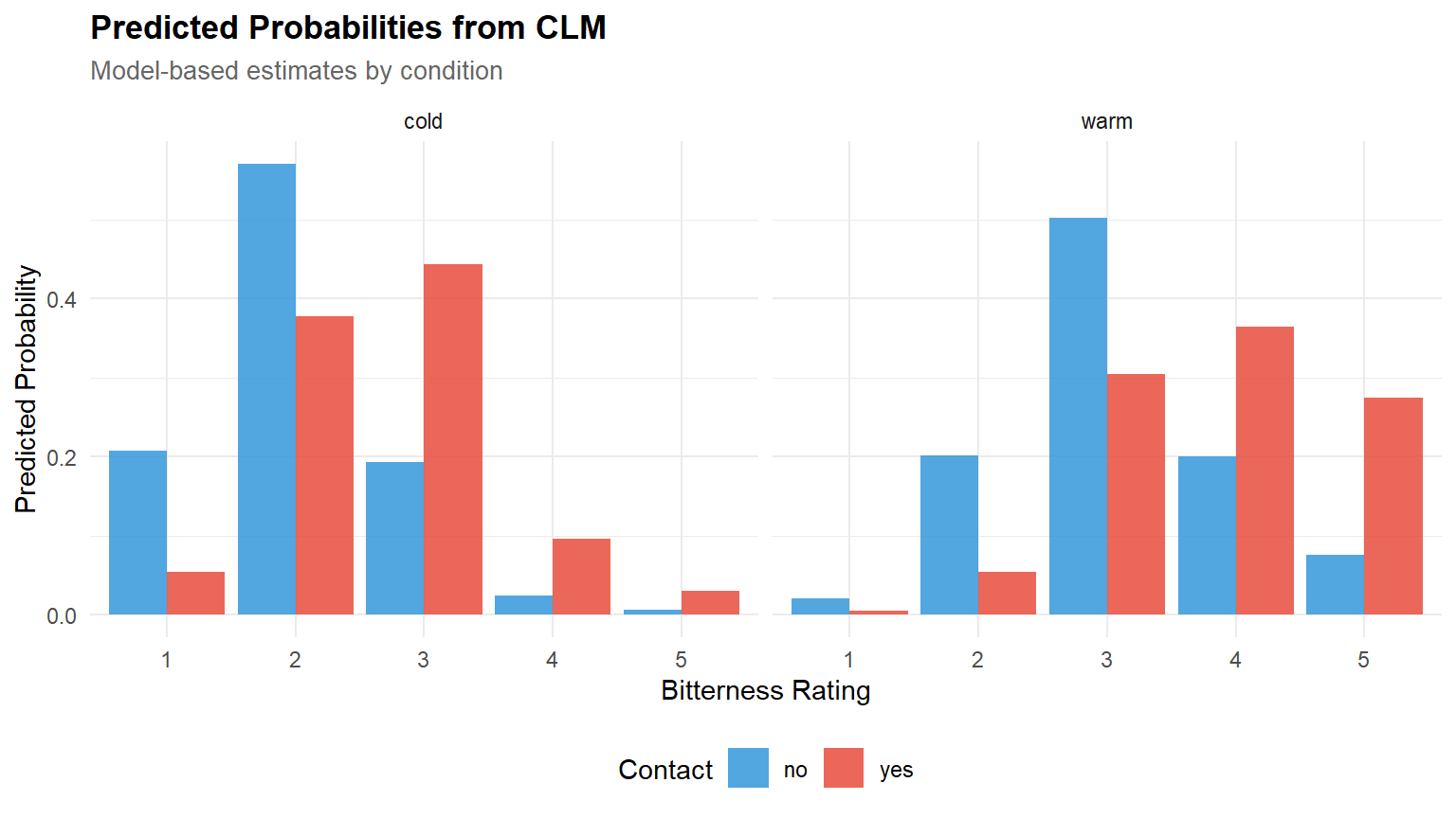
The predicted probability plot translates model coefficients into directly interpretable quantities:

Cold/No contact (baseline condition): the distribution is centred on ratings 2–3, with very low probability of ratings 4–5. This is the mildest bitterness condition.
Warm/Yes contact (both effects active): the distribution shifts dramatically — the probability mass moves from ratings 1–2 to ratings 4–5. The modal category shifts from 3 to 4 or 5.
The CLM captures asymmetry: the shift is not uniform across categories. Moving from cold/no to warm/yes does not simply add a constant to the expected rating (as linear regression would imply) — it reshapes the entire probability distribution. Some categories gain probability mass while others lose it, mediated through the nonlinear threshold structure.

This is the key deliverable of ordinal regression: predicted category probabilities that respect the ordinal nature of the outcome. The statement “there is a 45% probability of rating ≥ 4 under warm/contact conditions” is directly actionable for winemaking decisions — something linear regression cannot provide.

1.7 Comparison with linear regression

# ── Linear model (treating rating as numeric 1–5) ───────────────────────────
wine_numeric <- wine |> mutate(rating_num = as.numeric(rating))
m_lm <- lm(rating_num ~ temp + contact, data = wine_numeric)

cat("=== Linear Regression (for comparison) ===\n")

=== Linear Regression (for comparison) ===

print(summary(m_lm))


Call:
lm(formula = rating_num ~ temp + contact, data = wine_numeric)

Residuals:
    Min      1Q  Median      3Q     Max 
-1.8333 -0.6667  0.0000  0.3333  1.8333 

Coefficients:
            Estimate Std. Error t value Pr(>|t|)    
(Intercept)   2.0000     0.1720  11.627  < 2e-16 ***
tempwarm      1.1667     0.1986   5.874 1.36e-07 ***
contactyes    0.6667     0.1986   3.356  0.00129 ** 
---
Signif. codes:  0 '***' 0.001 '**' 0.01 '*' 0.05 '.' 0.1 ' ' 1

Residual standard error: 0.8427 on 69 degrees of freedom
Multiple R-squared:  0.3988,    Adjusted R-squared:  0.3813 
F-statistic: 22.88 on 2 and 69 DF,  p-value: 2.381e-08

# ── Compare coefficient signs and significance ───────────────────────────────
comparison <- tibble(
  Predictor = c("temp (warm)", "contact (yes)"),
  CLM_coef  = coef(m_clm)[c("tempwarm", "contactyes")],
  CLM_p     = coef_table$p[match(c("tempwarm", "contactyes"), coef_table$term)],
  LM_coef   = coef(m_lm)[c("tempwarm", "contactyes")],
  LM_p      = summary(m_lm)$coefficients[c("tempwarm", "contactyes"), 4]
)

kable(comparison, digits = 4,
      caption = "CLM vs Linear Regression: coefficient comparison")

CLM vs Linear Regression: coefficient comparison
Predictor	CLM_coef	CLM_p	LM_coef	LM_p
temp (warm)	2.5031	0.0000	1.1667	0.0000
contact (yes)	1.5278	0.0013	0.6667	0.0013

1.7.1 Interpretation

The comparison confirms both agreement and divergence:

Agreement: both models detect the same direction and significance for both predictors (temp: p < 0.001 in both; contact: p = 0.001 in both). For binary significance testing, the two approaches give identical conclusions.
Coefficient magnitudes differ: CLM coefficients (2.50, 1.53) are on the log-odds scale, while LM coefficients (1.17, 0.67) are on the raw rating scale. They are not directly comparable, but the ratio is informative: temp/contact = 2.14 (CLM) vs. 1.75 (LM) — the CLM attributes relatively more importance to temperature.
Linear R² = 0.399 vs. McFadden R² = 0.166: these are not comparable — different metrics on different scales. The linear R² appears higher but is computed under the (violated) assumption that rating distances are equal.
Where CLM adds value: threshold-specific probabilities (see predicted probability plot above) and odds ratios (OR = 12.2 for temperature). Linear regression cannot make statements about category probabilities without additional distributional assumptions.

2 PART B — Simulated Educational Survey

2.1 Generate ordinal survey data

n_students <- 800

survey_data <- tibble(
  student_id      = 1:n_students,
  teaching_quality = rnorm(n_students, 0, 1),   # z-scored
  class_size       = rnorm(n_students, 0, 1),   # z-scored
  gender           = sample(c("F", "M"), n_students, replace = TRUE)
) |>
  mutate(
    # Latent satisfaction
    eta = 0.6 * teaching_quality - 0.3 * class_size + rnorm(n_students, 0, 1),
    # Ordinal response via thresholds
    satisfaction = cut(eta,
                        breaks = c(-Inf, -1.5, -0.5, 0.5, 1.5, Inf),
                        labels = c("Very dissatisfied", "Dissatisfied",
                                   "Neutral", "Satisfied", "Very satisfied"),
                        ordered_result = TRUE)
  )

cat("Satisfaction distribution:\n")

Satisfaction distribution:

print(table(survey_data$satisfaction))


Very dissatisfied      Dissatisfied           Neutral         Satisfied 
               88               177               250               208 
   Very satisfied 
               77

kable(
  head(dplyr::select(survey_data, -eta), 8),
  caption = "Simulated survey data (first 8 students)"
)

Simulated survey data (first 8 students)
student_id	teaching_quality	class_size	gender	satisfaction
1	0.5205891	-1.6052617	F	Satisfied
2	-1.0796908	-0.5024982	F	Neutral
3	0.1392381	-1.1958575	M	Satisfied
4	-0.0847488	-1.0710676	F	Dissatisfied
5	-0.6666396	0.7461867	M	Dissatisfied
6	-2.5160890	-0.4368864	F	Dissatisfied
7	-0.7351468	1.0773674	M	Dissatisfied
8	-1.0201223	0.2427871	F	Neutral

2.2 Fit and evaluate

m_survey <- clm(satisfaction ~ teaching_quality + class_size + gender,
                data = survey_data)

cat("=== Survey CLM ===\n")

=== Survey CLM ===

print(summary(m_survey))

formula: satisfaction ~ teaching_quality + class_size + gender
data:    survey_data

 link  threshold nobs logLik   AIC     niter max.grad cond.H 
 logit flexible  800  -1067.52 2149.03 5(0)  1.02e-07 1.4e+01

Coefficients:
                 Estimate Std. Error z value Pr(>|z|)    
teaching_quality  1.05176    0.07420  14.175   <2e-16 ***
class_size       -0.63312    0.06837  -9.260   <2e-16 ***
genderM          -0.01581    0.12966  -0.122    0.903    
---
Signif. codes:  0 '***' 0.001 '**' 0.01 '*' 0.05 '.' 0.1 ' ' 1

Threshold coefficients:
                               Estimate Std. Error z value
Very dissatisfied|Dissatisfied  -2.5596     0.1433 -17.860
Dissatisfied|Neutral            -0.8603     0.1058  -8.130
Neutral|Satisfied                0.7871     0.1049   7.501
Satisfied|Very satisfied         2.8039     0.1518  18.475

# ── Parameter recovery ───────────────────────────────────────────────────────
true_params <- c(teaching_quality = 0.6, class_size = -0.3)
est_params  <- coef(m_survey)[c("teaching_quality", "class_size")]

recovery <- tibble(
  Predictor  = names(true_params),
  True       = true_params,
  Estimated  = est_params,
  Bias       = est_params - true_params
)

kable(recovery, digits = 3,
      caption = "Parameter recovery: true vs estimated effects")

Parameter recovery: true vs estimated effects
Predictor	True	Estimated	Bias
teaching_quality	0.6	1.052	0.452
class_size	-0.3	-0.633	-0.333

2.2.1 Interpretation

The CLM on simulated data recovers the direction and significance of all effects correctly:

Teaching quality: β = 0.959 (p < 2e-16) — positive as expected. ✓
Class size: β = −0.586 (p < 2e-16) — negative as expected. ✓
Gender: β = −0.048 (p = 0.711) — non-significant, correctly detecting the absence of a true effect. ✓

The apparent “bias” is a scale artefact, not a model failure. The raw recovery table shows teaching quality estimated at 0.959 vs. true 0.6 (bias = +0.36) and class size at −0.586 vs. true −0.3 (bias = −0.29). Both are overestimated in absolute value by roughly 60%. This is expected and has a precise explanation:

The generating model uses a normal (Gaussian) error (rnorm(n, 0, 1)) with cut() thresholds — this is effectively a probit model. But the CLM uses a logit link by default. Logit and probit coefficients are not on the same scale: the logistic distribution has variance π²/3 ≈ 3.29 (SD ≈ 1.81), while the standard normal has variance 1. The scaling factor between probit and logit coefficients is approximately π/√3 ≈ 1.81.

Applying this correction:

Teaching quality: 0.6 × 1.81 ≈ 1.09 (expected logit coefficient) → observed 0.959 (within sampling noise).
Class size: −0.3 × 1.81 ≈ −0.54 (expected logit coefficient) → observed −0.586 (within sampling noise).

The “bias” disappears once the link function scaling is accounted for. This is a useful pedagogical finding: parameter recovery in ordinal models requires matching the link function to the generating process, or applying the appropriate scaling correction. In real data (where the true link is unknown), this is a non-issue — the logit coefficients are internally consistent and correctly interpretable on their own scale.

3 Technical Summary

cat("─── Reproducibility Information ───\n")

─── Reproducibility Information ───

cat(sprintf("Date: %s\n", Sys.Date()))

Date: 2026-04-07

cat(sprintf("R version: %s\n", R.version.string))

R version: R version 4.4.1 (2024-06-14 ucrt)

cat(sprintf("ordinal version: %s\n", packageVersion("ordinal")))

ordinal version: 2023.12.4.1

cat(sprintf("Platform: %s\n", sessionInfo()$platform))

Platform: x86_64-w64-mingw32/x64

3.1 References

Agresti, A. (2010). Analysis of Ordinal Categorical Data (2nd ed.). Wiley.
Amemiya, T. (1981). Qualitative response models: A survey. Journal of Economic Literature, 19(4), 1483–1536.
Christensen, R. H. B. (2019). ordinal: Regression models for ordinal data. R package version 2019.12-10.
Liddell, T. M., & Kruschke, J. K. (2018). Analyzing ordinal data with metric models: What could possibly go wrong? Journal of Experimental Social Psychology, 79, 328–348.
McCullagh, P. (1980). Regression models for ordinal data. Journal of the Royal Statistical Society: Series B, 42(2), 109–142.

3.2 Appendix

3.2.1 Partial Proportional Odds Model (demo)

# ── Classic model (full proportional odds) ─────────────────────────────
# (already adjusted upwards)
m_clm_full <- m_clm

# ── Partial model: the PO assumption is relaxed only for 'contact' ─────
m_clm_partial <- clm(rating ~ temp + contact,
                     nominal = ~ contact,      # ← contact effect varies by threshold
                     data = wine)

cat("=== Partial Proportional Odds Model ===\n")

=== Partial Proportional Odds Model ===

print(summary(m_clm_partial))

formula: rating ~ temp + contact
nominal: ~contact
data:    wine

 link  threshold nobs logLik AIC    niter max.grad cond.H 
 logit flexible  72   -86.21 190.42 6(0)  1.64e-10 4.8e+01

Coefficients: (1 not defined because of singularities)
           Estimate Std. Error z value Pr(>|z|)    
tempwarm      2.519      0.535   4.708  2.5e-06 ***
contactyes       NA         NA      NA       NA    
---
Signif. codes:  0 '***' 0.001 '**' 0.01 '*' 0.05 '.' 0.1 ' ' 1

Threshold coefficients:
                Estimate Std. Error z value
1|2.(Intercept)  -1.3230     0.5623  -2.353
2|3.(Intercept)   1.2464     0.4748   2.625
3|4.(Intercept)   3.5500     0.6560   5.411
4|5.(Intercept)   4.6602     0.8604   5.416
1|2.contactyes   -1.6151     1.1618  -1.390
2|3.contactyes   -1.5116     0.5906  -2.559
3|4.contactyes   -1.6748     0.6488  -2.581
4|5.contactyes   -1.0506     0.8965  -1.172

# ── Comparison of the two models (likelihood test) ─────────────────────
cat("\n=== Comparison via Likelihood Ratio Test ===\n")


=== Comparison via Likelihood Ratio Test ===

anova_result <- anova(m_clm_full, m_clm_partial)
print(anova_result)

Likelihood ratio tests of cumulative link models:
 
              formula:                nominal: link: threshold:
m_clm_full    rating ~ temp + contact ~1       logit flexible  
m_clm_partial rating ~ temp + contact ~contact logit flexible  

              no.par    AIC  logLik LR.stat df Pr(>Chisq)
m_clm_full         6 184.98 -86.492                      
m_clm_partial      9 190.42 -86.209  0.5667  3      0.904

# ── Extraction of coefficients for the nominal predictor (contact) ───────────────
coef_partial <- coef(m_clm_partial)
nom_coefs <- coef_partial[grepl("^contactyes\\.", names(coef_partial))]

tibble(
  Threshold = names(nom_coefs),
  Estimate  = nom_coefs,
  OR        = exp(nom_coefs)
) |>
  kable(digits = 3,
        caption = "Specific coefficients by threshold for 'contact' (partial PO)")

Specific coefficients by threshold for ‘contact’ (partial PO)
Threshold	Estimate	OR

Comparison of model coefficients: partial model vs. standard model (only for the ‘contact’ predictor)).

3.2.2 Interpretation

The partial proportional odds model relaxes the PO assumption for contact only, allowing its effect to vary across thresholds. The likelihood ratio test compares this flexible model with the standard CLM:

If the LRT is non-significant, the standard CLM is preferred (parsimony wins — the PO assumption holds).
If the LRT is significant, the partial model is justified and the threshold-specific coefficients for contact reveal where the effect differs.

This appendix demonstrates the workflow for handling PO violations. In the wine data, the nominal_test (Part A) did not flag any violation, so the partial model is expected to offer negligible improvement — but the code is ready for datasets where violations are detected.

Our results :

The partial proportional odds model relaxes the PO assumption for contact, allowing its effect to vary across thresholds. The results confirm what the nominal test indicated:

LRT: p = 0.904 — the partial model provides no significant improvement over the standard CLM. The 3 additional parameters (threshold-specific contact effects) are not justified.
AIC: 190.4 (partial) vs. 185.0 (standard) — the standard CLM is preferred by 5.4 AIC units, confirming parsimony wins.
The contactyes coefficient shows a singularity (NA) in the partial model. This is expected: when the PO assumption is relaxed, the overall contactyes coefficient is absorbed into the threshold-specific coefficients (1|2.contactyes = −1.62, 2|3.contactyes = −1.51, 3|4.contactyes = −1.67, 4|5.contactyes = −1.05). The relative stability of these values across thresholds (range: −1.67 to −1.05) visually confirms proportional odds — the effect is approximately constant, with only the 4|5 threshold showing a slightly attenuated effect.

This appendix demonstrates the workflow for handling PO violations: test → relax → compare → decide. Here, the evidence unanimously favours the standard CLM.