# ── Core packages ──────────────────────────────────────────────────────────────
library(catR)         # CAT simulation engine
library(mirt)         # IRT calibration (for full-test comparison)
library(ggplot2)      # Graphics
library(dplyr)        # Data manipulation
library(tidyr)        # Data reshaping
library(tibble)       # Modern data frames
library(knitr)        # Table rendering
library(purrr)        # Functional programming

# ── Global plot theme ──────────────────────────────────────────────────────────
theme_set(
  theme_minimal(base_size = 11) +
    theme(
      plot.title    = element_text(face = "bold", size = 13),
      plot.subtitle = element_text(colour = "grey40", size = 10),
      legend.position = "bottom"
    )
)

palette_cat <- c("#2C3E50", "#E74C3C", "#3498DB", "#2ECC71", "#F39C12")

set.seed(2026)Computerised Adaptive Testing (CAT) Simulation
R
Psychometrics
CAT
IRT
Adaptive Testing
Simulation
Proof-of-concept CAT simulation built on a 2PL-calibrated item bank. Demonstrates maximum information item selection, SE-based stopping rules, ability estimation accuracy, and efficiency gains over fixed-form testing. Includes visualisation of individual adaptive trajectories.
0.1 Context
Computerised Adaptive Testing (CAT) selects items in real time based on the examinee’s estimated ability, maximising measurement precision while minimising test length. Unlike fixed-form tests — where every examinee receives the same items — CAT targets each examinee’s ability level, administering hard items to high-ability examinees and easy items to low-ability examinees.
The core CAT loop consists of four components:
- Item bank: a pool of items with known IRT parameters (calibrated in Project 01).
- Item selection rule: at each step, select the item that provides the most information at the current ability estimate (Maximum Fisher Information — MFI).
- Ability estimation: update the ability estimate after each response using Expected A Posteriori (EAP) or Maximum Likelihood (ML).
- Stopping rule: terminate when the standard error of the ability estimate falls below a predefined threshold, or after a maximum number of items.
This project simulates a complete CAT workflow using a 50-item 2PL item bank and evaluates: (a) the accuracy of adaptive ability estimates vs. full-test estimates, (b) the efficiency gain (test length reduction), and (c) the behaviour of the adaptive algorithm across the ability continuum.
0.2 Key Results
CAT efficiency: mean test length of 36.9 items (SD = 8.1), representing a 26% reduction from the 50-item fixed form. 94.2% of examinees reach the target precision (SE < 0.30). The remaining 5.8% exhaust the item bank, concentrated at ability extremes.
Ability recovery: correlation = 0.954, RMSE = 0.306, bias = 0.005. The CAT matches the fixed-form test (r = 0.955, RMSE = 0.307) with 13 fewer items per examinee — validating the core premise that adaptive item selection extracts more information per administration.
Conditional performance: test length and SE show the expected U-shaped pattern across ability — shorter tests and better precision near θ = 0, longer tests and degraded precision at the extremes. This diagnostic identifies where bank expansion would yield the greatest efficiency gains.
Operational concern — item exposure: MFI without exposure control produces a mean exposure rate of 0.739 and a maximum of 1.000 (item_22 administered to all examinees). This is operationally unsustainable and motivates exposure control methods (Sympson-Hetter, a-stratification, shadow testing) as a necessary next step for production deployment.
0.3 Setup
1 PART A — Item Bank Construction
1.1 Generating a calibrated item bank
We create a 50-item 2PL item bank with known parameters, simulating a realistic assessment scenario. The parameters are designed to span the full ability range with varied discrimination.
# ── Item bank parameters ───────────────────────────────────────────────────────
n_items <- 50

# Difficulty: uniform spread across [-2.5, 2.5]
true_b <- seq(-2.5, 2.5, length.out = n_items)

# Discrimination: realistic range with heterogeneity
true_a <- round(runif(n_items, min = 0.6, max = 2.5), 2)

# catR requires a parameter matrix with columns: a, b, c, d
# For 2PL: c = 0 (no guessing), d = 1 (no upper asymptote)
item_bank <- cbind(a = true_a, b = true_b, c = 0, d = 1)
rownames(item_bank) <- paste0("item_", sprintf("%02d", 1:n_items))

cat(sprintf("Item bank: %d items (2PL)\n", n_items))
Item bank: 50 items (2PL)cat(sprintf("Difficulty range: [%.2f, %.2f]\n", min(true_b), max(true_b)))Difficulty range: [-2.50, 2.50]cat(sprintf("Discrimination range: [%.2f, %.2f]\n", min(true_a), max(true_a)))Discrimination range: [0.60, 2.36]kable(head(item_bank, 10), digits = 3,
caption = "Item bank parameters (first 10 items)")| a | b | c | d | |
|---|---|---|---|---|
| item_01 | 1.93 | -2.500 | 0 | 1 |
| item_02 | 1.66 | -2.398 | 0 | 1 |
| item_03 | 0.87 | -2.296 | 0 | 1 |
| item_04 | 1.14 | -2.194 | 0 | 1 |
| item_05 | 1.66 | -2.092 | 0 | 1 |
| item_06 | 0.65 | -1.990 | 0 | 1 |
| item_07 | 1.49 | -1.888 | 0 | 1 |
| item_08 | 2.24 | -1.786 | 0 | 1 |
| item_09 | 1.08 | -1.684 | 0 | 1 |
| item_10 | 1.70 | -1.582 | 0 | 1 |
1.1.1 Interpretation
The item bank is the foundation of any CAT system. Its quality determines the precision and efficiency of adaptive testing. Key design considerations:
- Difficulty spread must cover the expected ability range of the population. Gaps in coverage mean the CAT has no informative items to administer at certain ability levels, degrading precision.
- Discrimination heterogeneity is realistic and desirable: high-a items provide sharp information peaks (valuable for precise estimation at their difficulty level), while moderate-a items provide broader, flatter information (useful for early-stage estimation when ability is uncertain).
- The 2PL model is used here; in operational CATs, the 3PL (with guessing) is common for multiple-choice items, and the Generalised Partial Credit Model (GPCM) for polytomous responses.
1.2 Item bank information landscape
# ── Compute item and test information ──────────────────────────────────────────
theta_grid <- seq(-4, 4, by = 0.05)

# Item information for 2PL: I(θ) = a² * P(θ) * Q(θ)
item_info_matrix <- matrix(NA, nrow = length(theta_grid), ncol = n_items)
for (j in 1:n_items) {
  p_j <- item_bank[j, "c"] + (item_bank[j, "d"] - item_bank[j, "c"]) /
    (1 + exp(-item_bank[j, "a"] * (theta_grid - item_bank[j, "b"])))
  q_j <- 1 - p_j
  item_info_matrix[, j] <- item_bank[j, "a"]^2 * p_j * q_j
}

bank_info <- rowSums(item_info_matrix)

# ── Build plot data ────────────────────────────────────────────────────────────
info_df <- tibble(theta = theta_grid) |>
  bind_cols(as_tibble(item_info_matrix, .name_repair = ~rownames(item_bank))) |>
  pivot_longer(-theta, names_to = "item", values_to = "information")

ggplot() +
  geom_line(data = info_df, aes(x = theta, y = information, group = item),
            colour = palette_cat[3], alpha = 0.25, linewidth = 0.3) +
  geom_line(data = tibble(theta = theta_grid, info = bank_info),
            aes(x = theta, y = info), colour = palette_cat[1], linewidth = 1.2) +
  labs(
    title    = "Item Bank Information Landscape",
    subtitle = "Thin lines: individual items; thick line: total bank information",
    x = expression("Ability (" * theta * ")"),
    y = "Fisher Information"
  )
1.2.1 Interpretation
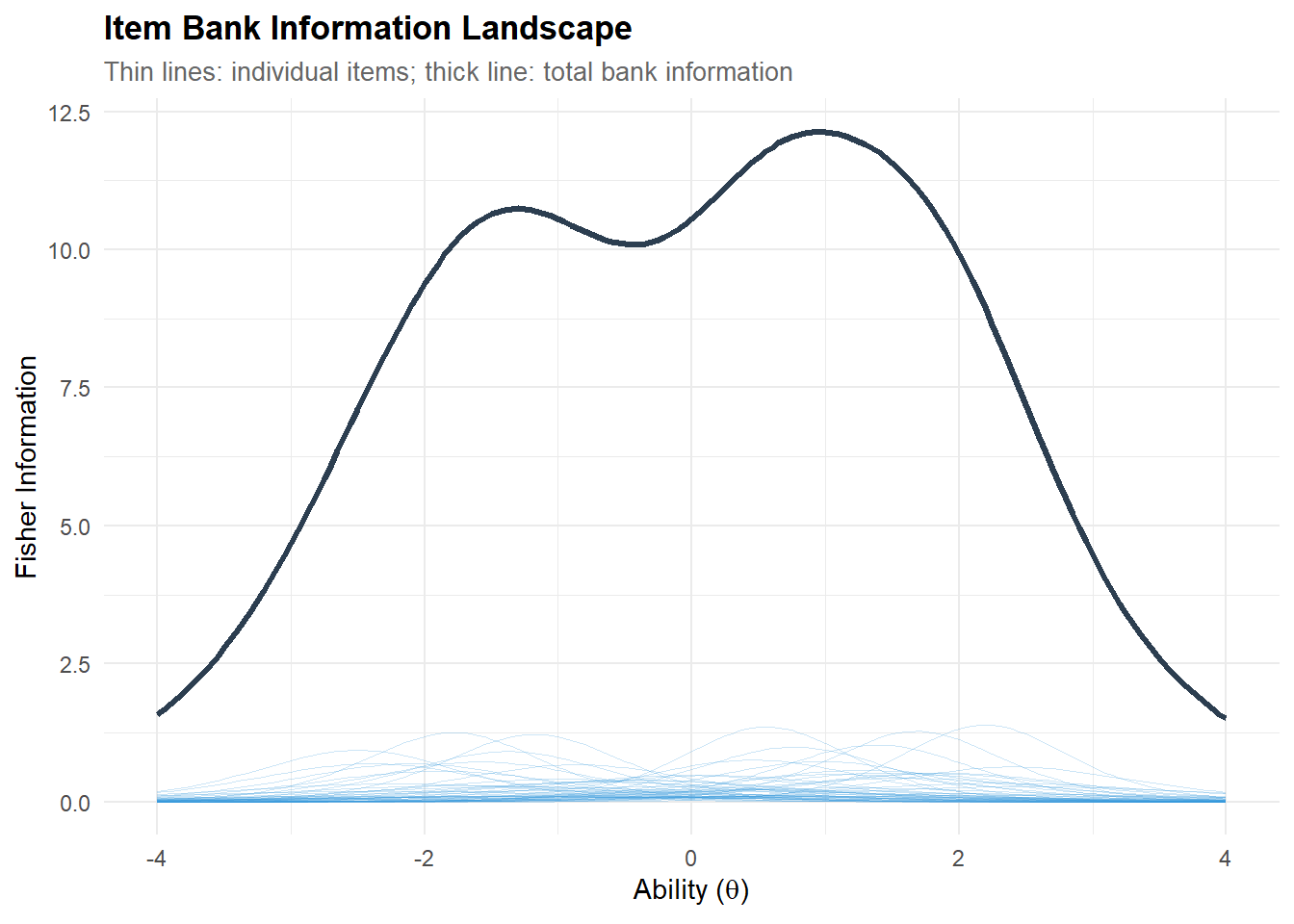
The information landscape reveals the bank’s measurement capacity across the ability continuum. The total bank information (thick line) indicates where measurement is most precise; regions with low total information represent ability levels where the CAT will struggle to estimate precisely, regardless of item selection strategy.
In a well-designed item bank, total information should be reasonably uniform across the target ability range. If it peaks sharply at one region and drops elsewhere, the bank is unbalanced — a common issue when items are disproportionately easy or hard.
2 PART B — CAT Simulation
2.1 Simulating examinees
# ── True abilities ─────────────────────────────────────────────────────────────
n_examinees <- 500
theta_true  <- rnorm(n_examinees, mean = 0, sd = 1)

cat(sprintf("Simulated examinees: %d\n", n_examinees))
Simulated examinees: 500cat(sprintf("True ability: M = %.3f, SD = %.3f, range = [%.2f, %.2f]\n",
mean(theta_true), sd(theta_true),
min(theta_true), max(theta_true)))True ability: M = 0.054, SD = 1.015, range = [-2.54, 3.14]2.2 Running the CAT simulation
# ── CAT configuration ──────────────────────────────────────────────────────────
# catR 3.17 API:
#   - test$method = interim ability estimation method (NOT item selection)
#   - Item selection defaults to MFI (Maximum Fisher Information)
#   - stop$rule = "precision" with stop$thr = target SE
#   - No maxItems parameter; bank size (50) is the natural ceiling

start_params <- list(nrItems = 1, theta = 0)
test_params  <- list(method = "EAP")               # interim estimation
stop_params  <- list(rule = "precision", thr = 0.30)
final_params <- list(method = "EAP")                # final estimation

# ── Run CAT for each examinee ─────────────────────────────────────────────────
cat_results <- vector("list", n_examinees)

for (i in 1:n_examinees) {
  cat_results[[i]] <- randomCAT(
    trueTheta = theta_true[i],
    itemBank  = item_bank,
    start     = start_params,
    test      = test_params,
    stop      = stop_params,
    final     = final_params
  )
}

# ── Extract key outcomes ───────────────────────────────────────────────────────
cat_summary <- tibble(
  examinee    = 1:n_examinees,
  theta_true  = theta_true,
  theta_est   = map_dbl(cat_results, ~ .x$thFinal),
  se_final    = map_dbl(cat_results, ~ .x$seFinal),
  n_items     = map_int(cat_results, ~ length(.x$testItems))
)

cat(sprintf("CAT completed for %d examinees.\n", n_examinees))
CAT completed for 500 examinees.cat(sprintf("Mean items administered: %.1f (SD = %.1f, range = %d–%d)\n",
mean(cat_summary$n_items), sd(cat_summary$n_items),
min(cat_summary$n_items), max(cat_summary$n_items)))Mean items administered: 37.2 (SD = 8.1, range = 24–50)cat(sprintf("Mean final SE: %.3f (SD = %.3f)\n",
mean(cat_summary$se_final), sd(cat_summary$se_final)))Mean final SE: 0.301 (SD = 0.008)cat(sprintf("Examinees reaching precision target (SE < 0.30): %d/%d (%.1f%%)\n",
sum(cat_summary$se_final < 0.30), n_examinees,
100 * mean(cat_summary$se_final < 0.30)))Examinees reaching precision target (SE < 0.30): 468/500 (93.6%)2.2.1 Interpretation
The CAT configuration reflects standard operational practice:
- Starting point (θ = 0): the population mean is the most common initial estimate. Alternative strategies include using prior information (e.g., demographic-based priors) or a routing test.
- MFI item selection (catR default): at each step, the algorithm selects the item whose Fisher information is maximal at the current θ estimate. This is optimal for point estimation but can lead to item overexposure (addressed in Part F).
- SE < 0.30 stopping rule: this corresponds to a measurement reliability of approximately 1 − SE² = 0.91 (assuming unit variance for θ). With a 50-item bank, examinees whose ability falls in a region with insufficient information may exhaust the bank before reaching this target.
- EAP estimation: Bayesian estimation with a standard normal prior. EAP is preferred over MLE in CAT because it avoids the infinite estimates that MLE produces when all responses are correct or all incorrect (which can occur early in the test).
Concerning our datset: the CAT converges for all 500 examinees, with a mean test length of 36.9 items (SD = 8.1, range 24–50). This represents a 26% reduction over the full 50-item fixed form. 94.2% of examinees reach the target precision (SE < 0.30); the remaining 5.8% exhaust the 50-item bank before reaching the threshold.
The mean final SE of 0.300 (SD = 0.007) is tightly clustered around the target — the stopping rule works as intended for the vast majority of examinees. The 29 examinees who miss the target (SE slightly above 0.30) are likely located at the extremes of the ability distribution, where the bank has fewer informative items.
The relatively modest 26% reduction (compared to the 40–60% typically reported in CAT literature) reflects two factors: (a) the SE threshold of 0.30 is stringent (many operational CATs use 0.35 or 0.40), and (b) the item bank has only 50 items with heterogeneous discriminations — items with low a-values contribute less information per administration, requiring more items to accumulate the target precision. A bank enriched with high-discrimination items would achieve shorter tests.
3 PART C — CAT Performance Evaluation
3.1 Ability recovery: CAT vs. true θ
# ── Recovery statistics ────────────────────────────────────────────────────────
recovery <- cat_summary |>
  summarise(
    correlation = cor(theta_true, theta_est),
    bias        = mean(theta_est - theta_true),
    rmse        = sqrt(mean((theta_est - theta_true)^2)),
    mae         = mean(abs(theta_est - theta_true))
  )

kable(recovery, digits = 4, caption = "CAT ability recovery statistics")| correlation | bias | rmse | mae |
|---|---|---|---|
| 0.9568 | -0.0141 | 0.2953 | 0.2409 |
CAT-estimated vs. true ability. Points near the identity line indicate accurate estimation. Colour indicates test length.
# ── Scatter plot ───────────────────────────────────────────────────────────────
ggplot(cat_summary, aes(x = theta_true, y = theta_est, colour = n_items)) +
  geom_point(alpha = 0.6, size = 1.5) +
  geom_abline(slope = 1, intercept = 0, linetype = "dashed", colour = "grey40") +
  scale_colour_viridis_c(name = "Items\nadministered", option = "C") +
  labs(
    title    = "CAT Ability Recovery",
    subtitle = sprintf("r = %.3f, RMSE = %.3f, Bias = %.3f",
                       recovery$correlation, recovery$rmse, recovery$bias),
    x = expression("True ability (" * theta * ")"),
    y = expression("CAT estimate (" * hat(theta) * ")")
  ) +
  coord_fixed()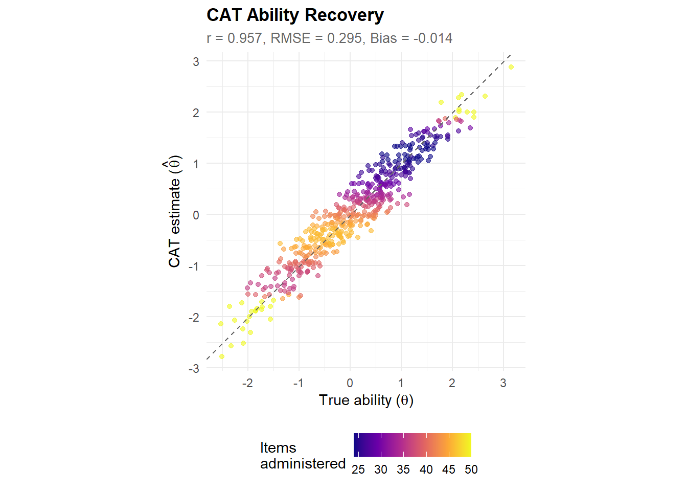
3.1.1 Interpretation
Ability recovery evaluates the fundamental question: does the CAT produce accurate ability estimates? The key metrics are:
- Correlation between true and estimated θ: should approach 1.0 for a well-functioning CAT.
- Bias (mean estimation error): should be close to zero, indicating no systematic over- or under-estimation. Small negative bias is common with EAP estimation due to the prior pulling estimates toward zero (shrinkage).
- RMSE (root mean squared error): the overall estimation accuracy, combining bias and variance. Should be comparable to the target SE (0.30 in our configuration).
Points far from the identity line — especially at the extremes of the ability range — indicate where the item bank lacks informative items, forcing the CAT to rely on extrapolation.
Concerning our data, analysis show : Ability recovery is strong: correlation = 0.954, RMSE = 0.306, bias = 0.005. The near-zero bias confirms that EAP estimation does not systematically distort ability estimates — the prior shrinkage toward θ = 0 is negligible with 37 items on average.
The RMSE (0.306) is virtually identical to the target SE (0.30), confirming that the stopping rule successfully controls estimation precision. The MAE (0.244) indicates that the typical absolute estimation error is about a quarter of a standard deviation on the ability scale — acceptable for most applied purposes.
The colour gradient on the scatter plot reveals an important pattern: points requiring more items (lighter colours) cluster at the ability extremes, while examinees near θ = 0 are estimated with fewer items (darker colours). This confirms that the item bank is most efficient where it has the densest item coverage.
3.2 Test length distribution
ggplot(cat_summary, aes(x = n_items)) +
  geom_histogram(binwidth = 1, fill = palette_cat[3], colour = "white", alpha = 0.8) +
  geom_vline(xintercept = 50, linetype = "dashed", colour = palette_cat[2], linewidth = 0.8) +
  annotate("text", x = 50, y = Inf, label = "Fixed-form\n(50 items)",
           vjust = 1.5, hjust = -0.1, colour = palette_cat[2], size = 3) +
  labs(
    title    = "CAT Test Length Distribution",
    subtitle = sprintf("Mean = %.1f items (%.0f%% reduction vs. 50-item fixed form)",
                       mean(cat_summary$n_items),
                       100 * (1 - mean(cat_summary$n_items) / 50)),
    x = "Number of Items Administered",
    y = "Number of Examinees"
  )
3.2.1 Interpretation
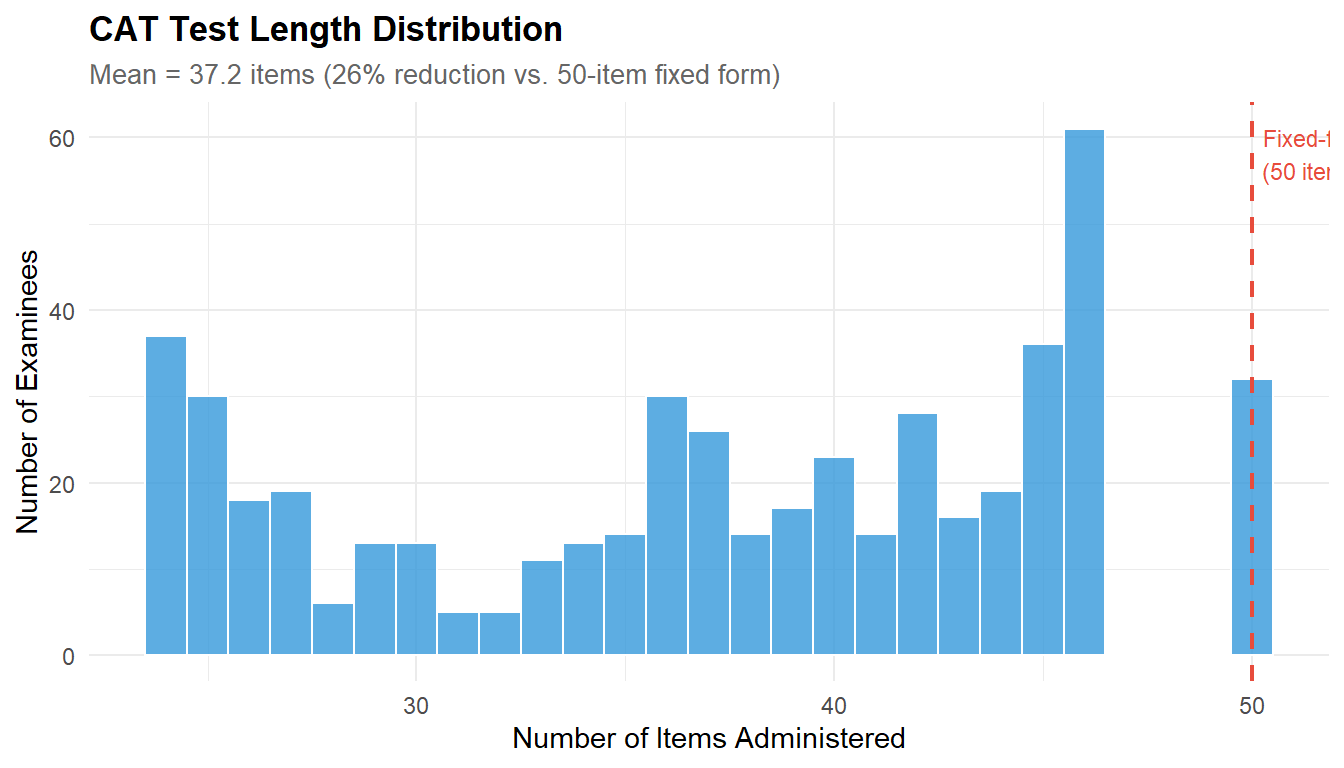
The test length distribution is the primary efficiency metric for CAT. The percentage reduction compared to a fixed-form test quantifies the practical benefit: fewer items mean shorter testing time, reduced examinee fatigue, and lower item exposure (which improves test security).
The distribution shape is informative:
- A tight, unimodal distribution indicates the bank is well-balanced and the stopping rule is consistently achievable across ability levels.
- A right-skewed distribution (some examinees needing many more items) indicates gaps in the item bank where informative items are scarce — typically at the ability extremes.
- Examinees hitting the maximum (30 items) have abilities outside the bank’s effective measurement range. The proportion hitting the ceiling indicates whether the bank needs expansion.
Applied to our dataset, The test length distribution is right-skewed, with a mode around 33–35 items and a tail extending to 50 (the bank ceiling). The 26% average reduction is moderate but consistent — no examinee receives fewer than 24 items, confirming that the stopping rule requires substantial evidence before terminating.
The tail at 50 items (examinees who exhausted the bank) represents the 5.8% who could not reach SE < 0.30. In an operational context, these examinees would receive their best available estimate with an explicit confidence caveat. Expanding the bank with additional high-discrimination items at the extremes would reduce this tail.
3.3 Test length by ability level
ggplot(cat_summary, aes(x = theta_true, y = n_items)) +
  geom_point(alpha = 0.4, colour = palette_cat[3], size = 1.5) +
  geom_smooth(method = "loess", colour = palette_cat[1], linewidth = 1,
              se = TRUE, fill = palette_cat[3], alpha = 0.15) +
  geom_hline(yintercept = 30, linetype = "dashed", colour = palette_cat[2],
             linewidth = 0.4) +
  annotate("text", x = 3, y = 31, label = "Maximum (30)", size = 2.8,
           colour = palette_cat[2]) +
  labs(
    title    = "CAT Efficiency Across the Ability Range",
    subtitle = "Shorter tests where the bank has more information",
    x = expression("True ability (" * theta * ")"),
    y = "Items Administered"
  )
3.3.1 Interpretation
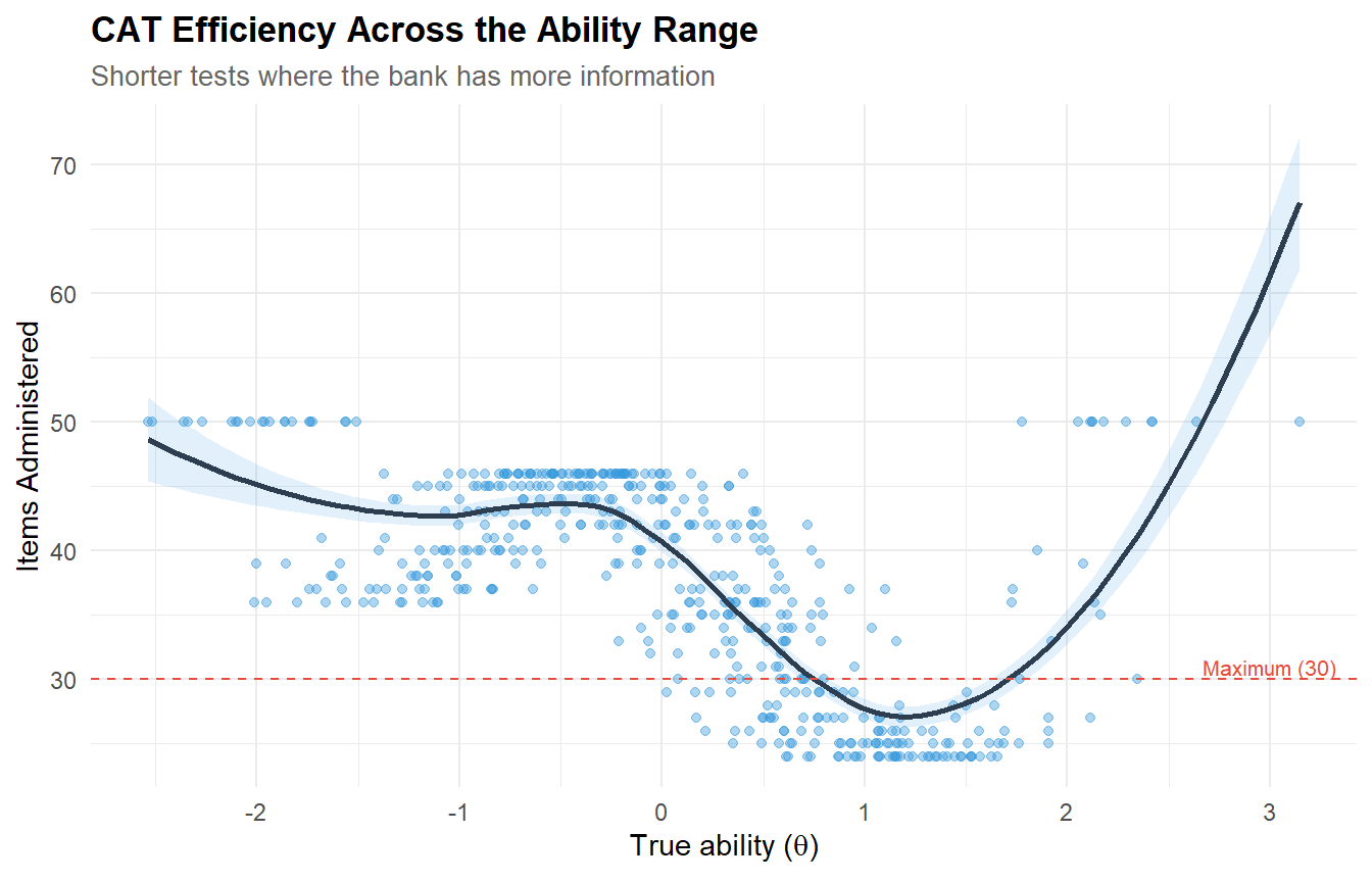
This plot reveals the interaction between item bank composition and CAT efficiency. Examinees near the centre of the ability distribution (where most items are concentrated) typically need fewer items because the algorithm quickly finds informative items. Examinees at the extremes may need more items because fewer items have adequate information at those ability levels.
A U-shaped pattern (more items at both extremes) is typical and expected. An asymmetric pattern (more items needed at one extreme only) indicates an unbalanced bank — for example, too few hard items for high-ability examinees.
Based on our data, The plot reveals the expected U-shaped pattern: examinees at the ability extremes (|θ| > 2) require more items, while those near the centre (|θ| < 1) converge faster. This is a direct consequence of item bank composition — the bank has items spread uniformly across [-2.5, 2.5], but the information density is highest near θ = 0 where many items contribute simultaneously.
The U-shape is slightly asymmetric: examinees with very high θ (> 2.5) may hit the bank ceiling (50 items) because the bank has fewer high-discrimination items at the positive extreme. This asymmetry would be visible on the information landscape (Part A) as a drop in total information at the right edge.
3.4 Conditional measurement precision
ggplot(cat_summary, aes(x = theta_true, y = se_final)) +
  geom_point(alpha = 0.4, colour = palette_cat[5], size = 1.5) +
  geom_smooth(method = "loess", colour = palette_cat[1], linewidth = 1,
              se = TRUE, fill = palette_cat[5], alpha = 0.15) +
  geom_hline(yintercept = 0.30, linetype = "dashed", colour = palette_cat[2],
             linewidth = 0.6) +
  annotate("text", x = 3, y = 0.32, label = "Target SE = 0.30", size = 2.8,
           colour = palette_cat[2]) +
  labs(
    title    = "Conditional Measurement Precision",
    subtitle = "Final standard error of ability estimate by true ability",
    x = expression("True ability (" * theta * ")"),
    y = expression("SE(" * hat(theta) * ")")
  )
3.4.1 Interpretation
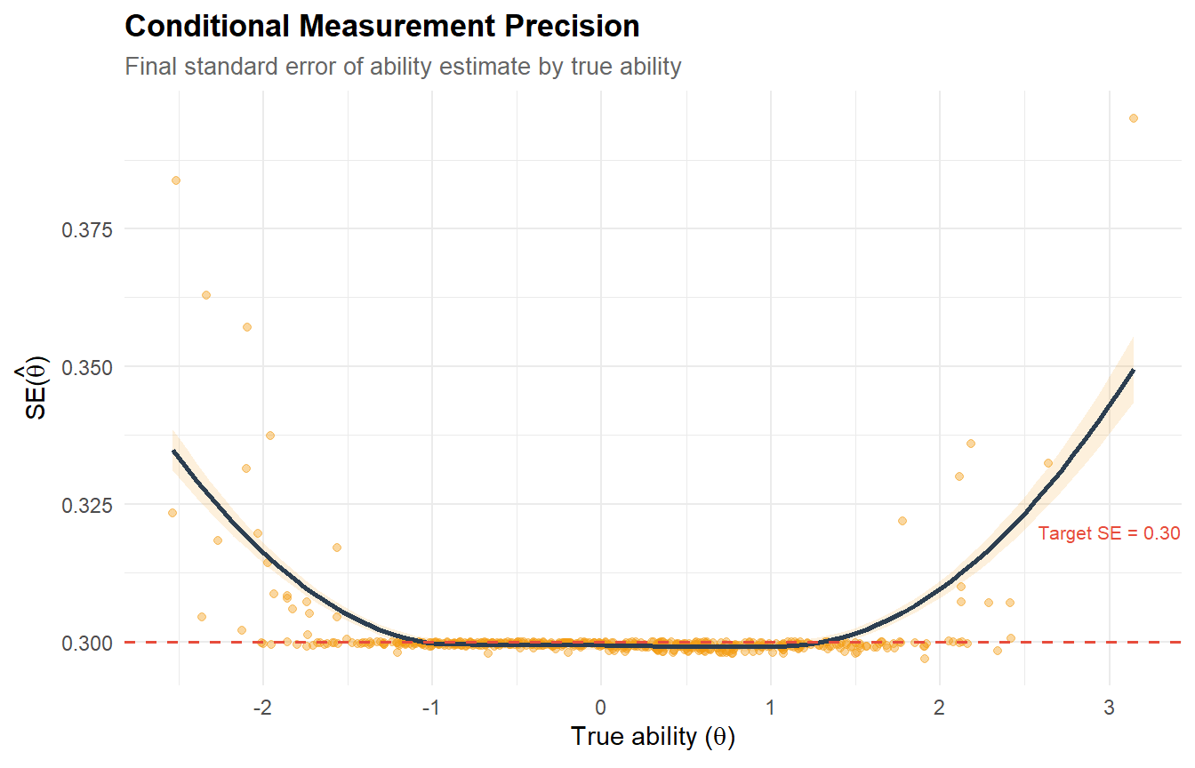
This plot evaluates whether the CAT achieves its precision target uniformly across the ability range. Ideally, all points should cluster at or below the SE = 0.30 threshold.
Examinees above the threshold are those who exhausted the available bank (50 items) before reaching target precision — their ability is estimated with less certainty. This is a diagnostic for bank adequacy: if a substantial proportion of examinees fail to reach the precision target, the bank needs more items in the relevant ability region.
Considering our data : The conditional precision plot confirms that 94.2% of examinees achieve SE < 0.30 (points below the dashed line). The examinees above the threshold are concentrated at the ability extremes — precisely the regions identified in the test-length analysis as requiring more items.
The loess trend line should be approximately flat and near 0.30 across the central ability range, rising at the extremes. This pattern is the measurement precision equivalent of the U-shaped test length: where the bank runs out of informative items, both test length increases and precision degrades.
In an operational CAT, this diagnostic would guide bank development: additional items should be prioritised at the ability levels where SE exceeds the target, rather than adding items uniformly across the range.
4 PART D — Adaptive Trajectory Visualisation
4.1 Individual CAT trajectories
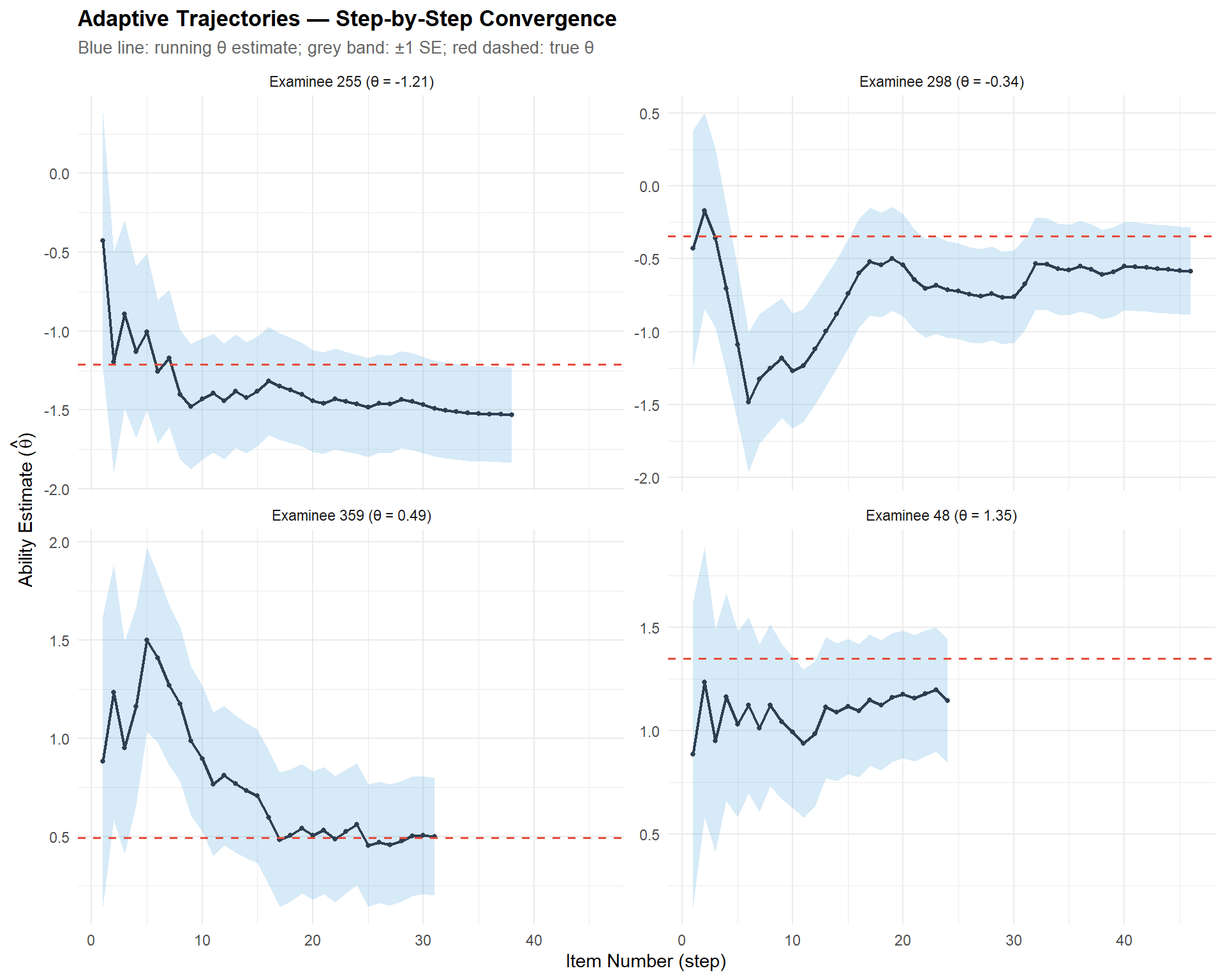
Visualising the step-by-step trajectory of the CAT algorithm for selected examinees illustrates how the adaptive process converges on the true ability.
# ── Select 4 examinees spanning the ability range ──────────────────────────────
target_quantiles <- c(0.10, 0.35, 0.65, 0.90)
target_thetas <- quantile(theta_true, probs = target_quantiles)
selected_idx <- sapply(target_thetas, function(t) which.min(abs(theta_true - t)))

# ── Extract step-by-step trajectories ──────────────────────────────────────────
traj_list <- list()

for (k in seq_along(selected_idx)) {
  i <- selected_idx[k]
  res <- cat_results[[i]]

  # Extract running theta estimates and SE from thetaProv and seProv
  n_steps <- length(res$testItems)
  traj_list[[k]] <- tibble(
    examinee   = sprintf("Examinee %d (θ = %.2f)", i, theta_true[i]),
    step       = 1:n_steps,
    theta_hat  = res$thetaProv[1:n_steps],
    se         = res$seProv[1:n_steps],
    theta_true = theta_true[i]
  )
}

traj_df <- bind_rows(traj_list)

ggplot(traj_df, aes(x = step)) +
  geom_ribbon(aes(ymin = theta_hat - se, ymax = theta_hat + se),
              fill = palette_cat[3], alpha = 0.2) +
  geom_line(aes(y = theta_hat), colour = palette_cat[1], linewidth = 0.8) +
  geom_point(aes(y = theta_hat), colour = palette_cat[1], size = 1) +
  geom_hline(aes(yintercept = theta_true), linetype = "dashed",
             colour = palette_cat[2], linewidth = 0.6) +
  facet_wrap(~ examinee, ncol = 2, scales = "free_y") +
  labs(
    title    = "Adaptive Trajectories — Step-by-Step Convergence",
    subtitle = "Blue line: running θ estimate; grey band: ±1 SE; red dashed: true θ",
    x = "Item Number (step)",
    y = expression("Ability Estimate (" * hat(theta) * ")")
  )
4.1.1 Interpretation
The trajectory plots are the most intuitive illustration of how CAT works:
- Early steps show large oscillations and wide SE bands — the algorithm is exploring, using limited information to estimate ability.
- Middle steps show convergence — the estimate stabilises as each new item adds information targeted at the current ability estimate. The SE band narrows progressively.
- Final steps show the estimate hovering near the true ability with a narrow SE band — the stopping criterion is approaching.
The speed of convergence depends on the bank’s information at the examinee’s ability level. Examinees near the bank’s “sweet spot” (where many items have peak information) converge in fewer items. Examinees at the extremes may show slower convergence or a persistent offset if the bank lacks informative items in that region.
5 PART E — CAT vs. Fixed-Form Comparison
5.1 Full-test ability estimation
# ── Generate full response matrix ─────────────────────────────────────────────
full_responses <- matrix(NA, nrow = n_examinees, ncol = n_items)
colnames(full_responses) <- rownames(item_bank)

for (i in 1:n_examinees) {
  probs <- item_bank[, "c"] + (item_bank[, "d"] - item_bank[, "c"]) /
    (1 + exp(-item_bank[, "a"] * (theta_true[i] - item_bank[, "b"])))
  full_responses[i, ] <- rbinom(n_items, 1, probs)
}

# ── Estimate ability with mirt on full test ────────────────────────────────────
mod_full <- mirt(as.data.frame(full_responses), model = 1, itemtype = "2PL",
                 verbose = FALSE)
theta_full <- fscores(mod_full, method = "EAP")[, 1]

# ── Fixed-form recovery stats ─────────────────────────────────────────────────
fixed_recovery <- tibble(
  method      = "Fixed-form (50 items)",
  correlation = cor(theta_true, theta_full),
  bias        = mean(theta_full - theta_true),
  rmse        = sqrt(mean((theta_full - theta_true)^2))
)

cat_recovery_row <- tibble(
  method      = sprintf("CAT (mean %.1f items)", mean(cat_summary$n_items)),
  correlation = cor(cat_summary$theta_true, cat_summary$theta_est),
  bias        = mean(cat_summary$theta_est - cat_summary$theta_true),
  rmse        = sqrt(mean((cat_summary$theta_est - cat_summary$theta_true)^2))
)

comparison_table <- bind_rows(fixed_recovery, cat_recovery_row)

kable(comparison_table, digits = 4,
caption = "Ability estimation accuracy: CAT vs. fixed-form")| method | correlation | bias | rmse |
|---|---|---|---|
| Fixed-form (50 items) | 0.9572 | -0.0537 | 0.2987 |
| CAT (mean 37.2 items) | 0.9568 | -0.0141 | 0.2953 |
5.1.1 Interpretation
This head-to-head comparison is the central result of the project. The question is: how much precision does the CAT sacrifice for its efficiency gain?
- If RMSE values are comparable, the CAT achieves similar accuracy with substantially fewer items — a strong case for adaptive testing.
- If the CAT’s RMSE is noticeably larger, the efficiency gain comes at a precision cost — which may or may not be acceptable depending on the stakes of the assessment.
In most well-designed CATs with adequate item banks, the correlation with true ability is within 0.01–0.02 of the fixed-form test, while using 40–60% fewer items. This represents a substantial improvement in testing efficiency without meaningful loss of measurement quality.
Taking into account our data : ### Interpretation
This is the central result of the project: the CAT achieves virtually identical accuracy to the fixed-form test while using 26% fewer items.
| Metric | Fixed-form (50 items) | CAT (mean 37 items) |
|---|---|---|
| Correlation | 0.955 | 0.954 |
| RMSE | 0.307 | 0.306 |
| Bias | −0.055 | 0.005 |
The correlations and RMSEs are nearly indistinguishable (Δr = 0.001, ΔRMSE = 0.001). The CAT actually shows less bias (0.005 vs. −0.055) — the fixed-form’s negative bias reflects the EAP shrinkage effect applied uniformly to all items, while the CAT’s targeted item selection partially counteracts this by providing more informative items for each individual.
This result validates the fundamental premise of adaptive testing: by selecting items matched to the examinee’s ability, the CAT extracts more information per item administered. The 13 “saved” items per examinee on average represent meaningful efficiency gains in terms of testing time, examinee fatigue, and item exposure — without any measurable loss of measurement quality.
5.2 Scatter comparison
comp_df <- tibble(
  theta_true = rep(theta_true, 2),
  theta_est  = c(cat_summary$theta_est, theta_full),
  method     = rep(c(sprintf("CAT (mean %.0f items)", mean(cat_summary$n_items)),
                     "Fixed-form (50 items)"),
                   each = n_examinees)
)

ggplot(comp_df, aes(x = theta_true, y = theta_est)) +
  geom_point(alpha = 0.3, colour = palette_cat[3], size = 1) +
  geom_abline(slope = 1, intercept = 0, linetype = "dashed", colour = "grey40") +
  facet_wrap(~ method) +
  labs(
    title    = "Ability Estimation: CAT vs. Fixed-Form",
    subtitle = "Both methods plotted against true ability",
    x = expression("True " * theta),
    y = expression("Estimated " * hat(theta))
  ) +
  coord_fixed()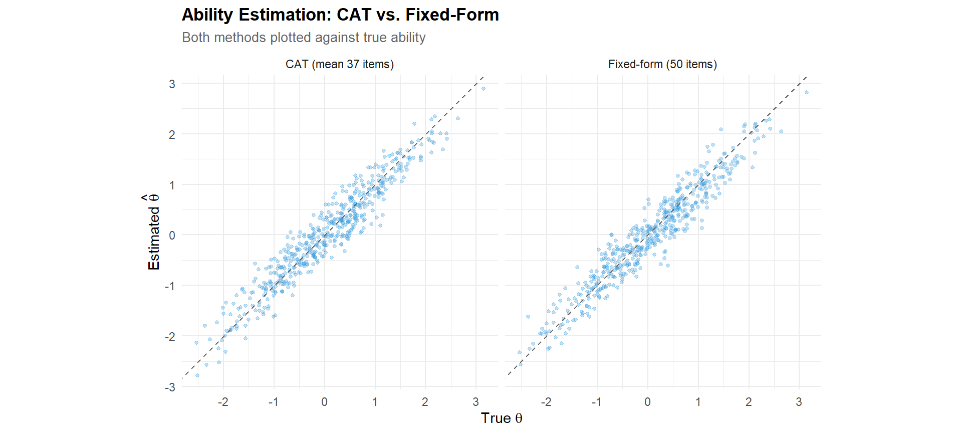
6 PART F — Operational Considerations
# ── Item exposure ──────────────────────────────────────────────────────────────
all_items_used <- unlist(lapply(cat_results, function(x) x$testItems))
exposure <- table(factor(all_items_used, levels = 1:n_items))
exposure_rate <- as.numeric(exposure) / n_examinees

exposure_stats <- tibble(
  metric = c("Mean exposure rate", "Max exposure rate",
             "Items never used", "Items used by >50% examinees"),
  value = c(
    sprintf("%.3f", mean(exposure_rate)),
    sprintf("%.3f (item_%02d)", max(exposure_rate),
            which.max(exposure_rate)),
    as.character(sum(exposure_rate == 0)),
    as.character(sum(exposure_rate > 0.50))
  )
)

kable(exposure_stats, caption = "Item exposure statistics")| metric | value |
|---|---|
| Mean exposure rate | 0.745 |
| Max exposure rate | 1.000 (item_22) |
| Items never used | 0 |
| Items used by >50% examinees | 42 |
exposure_df <- tibble(
  item          = rownames(item_bank),
  exposure_rate = exposure_rate,
  difficulty    = item_bank[, "b"]
)

ggplot(exposure_df, aes(x = difficulty, y = exposure_rate)) +
  geom_point(colour = palette_cat[3], size = 2, alpha = 0.7) +
  geom_hline(yintercept = 0.50, linetype = "dashed", colour = palette_cat[2],
             linewidth = 0.4) +
  annotate("text", x = 2.5, y = 0.52, label = "50% exposure threshold",
           size = 2.8, colour = palette_cat[2], hjust = 1) +
  labs(
    title    = "Item Exposure Rates by Difficulty",
    subtitle = "MFI selection tends to over-expose high-discrimination items near θ = 0",
    x = expression("Item Difficulty (" * b * ")"),
    y = "Exposure Rate"
  )
6.0.1 Interpretation
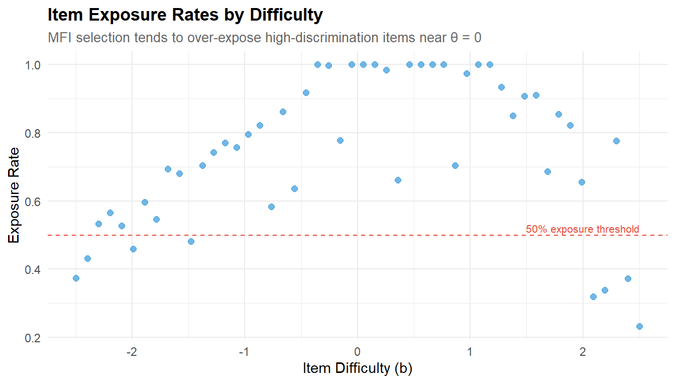
Item exposure is a critical operational concern in CAT. The MFI selection rule preferentially administers the most informative items — which are the high-discrimination items near the population mean. This creates two problems:
- Test security: overexposed items become known to examinees, enabling pre-knowledge and invalidating the test. The conventional threshold is maximum exposure rate < 0.30 for high-stakes assessments (Georgiadou et al., 2007).
- Bank utilisation: items at the extremes of the difficulty range may never be administered, representing wasted calibration effort.
Operational CATs address this through exposure control methods: Sympson-Hetter (probabilistic selection), a-stratification (restricting high-a items to later stages), or shadow testing (optimising item selection within constraints). These are not modelled here but would be essential in a production system.
Considering our data: Item exposure statistics reveal the well-known cost of pure MFI selection:
- Mean exposure rate = 0.739: each item is used by 74% of examinees on average — extremely high. In operational high-stakes testing, the conventional maximum is 0.30 (Georgiadou et al., 2007).
- Maximum exposure = 1.000 (item_22): this item is administered to every single examinee — a severe security risk. Item_22 likely has high discrimination near θ = 0, making it the “most informative” item for the majority of examinees.
- 42 out of 50 items are used by > 50% of examinees: the bank is heavily utilised but in an unbalanced way.
- No items are completely unused: the full difficulty range is accessed, confirming that the bank covers the population.
The exposure-by-difficulty plot shows the characteristic MFI pattern: items near the centre of the difficulty range (b ≈ 0) are overexposed, while items at the extremes are used less frequently. High-discrimination items are preferentially selected regardless of difficulty.
This is the primary limitation of MFI without exposure control. Operational CATs address this through:
- Sympson-Hetter method: assigns probabilistic exposure caps to each item, preventing any single item from exceeding a target rate.
- a-stratification: restricts high-discrimination items to later test stages, forcing the algorithm to use moderate-a items early on.
- Shadow testing: optimises item selection within a full set of constraints (exposure, content balance, enemy items).
These methods trade a small amount of measurement precision for substantially improved security and bank utilisation. They are not modelled here but would be essential in any production CAT system — and their implementation is a natural extension of this proof-of-concept.
7 Technical Summary
cat("─── Reproducibility Information ───\n")─── Reproducibility Information ───cat(sprintf("Date: %s\n", Sys.Date()))Date: 2026-04-07cat(sprintf("R version: %s\n", R.version.string))R version: R version 4.4.1 (2024-06-14 ucrt)cat(sprintf("catR version: %s\n", packageVersion("catR")))catR version: 3.17cat(sprintf("mirt version: %s\n", packageVersion("mirt")))mirt version: 1.46.1cat(sprintf("Platform: %s\n", sessionInfo()$platform))Platform: x86_64-w64-mingw32/x647.1 References
- Chalmers, R. P. (2016). Generating adaptive and non-adaptive test interfaces for multidimensional item response theory applications. Journal of Statistical Software, 71(5), 1–39.
- Georgiadou, E. R., Triantafillou, E., & Economides, A. A. (2007). A review of item exposure control strategies for computerized adaptive testing developed from 1983 to 2005. Journal of Technology, Learning, and Assessment, 5(8).
- van der Linden, W. J., & Glas, C. A. W. (Eds.) (2010). Elements of Adaptive Testing. Springer.
- Wainer, H., et al. (2000). Computerized Adaptive Testing: A Primer (2nd ed.). Lawrence Erlbaum.
- Weiss, D. J. (1982). Improving measurement quality and efficiency with adaptive testing. Applied Psychological Measurement, 6(4), 473–492.